#renv::restore() # Restore the project's dependencies from the lockfile to ensure that same package versions are used as in the original thesis.

library(caret) # For computing confusion matrices
library(harrypotter) # Only for colour scheme
library(here) # For path management
library(knitr) # Loaded to display the tables using the kable() function
library(paletteer) # For nice colours
library(readxl) # For the direct import of Excel files
library(tidyverse) # For everything else!Appendix D — Evaluation of the Multi-Feature Tagger of English (MFTE)
For more information on the tagger itself, as well as the evaluation data and methods, see Le Foll (2021) and https://github.com/elenlefoll/MultiFeatureTaggerEnglish.
Using the MFTE
The Multi-Feature Tagger of English (MFTE) Perl is free to use and was released under an Open Source licence. If you are interested in using the MFTE for your own project, I recommend using the latest version of the MFTE Python, which is much easier to use, can tag many more features, and also underwent a thorough evaluation. Note also that all future developments of the tool will be made on the MFTE Python. To find out more, see Le Foll & Shakir (2023) and https://github.com/mshakirDr/MFTE.
D.1 Set-up
The following packages must be installed and loaded to process the evaluation data.
Built with R 4.4.1
D.2 Data import from evaluation files
The data is imported directly from the Excel files in which the manual tag check and corrections was performed. A number of data wrangling steps need to be made for the data to be converted to a tidy format.
Code
# Function to import and wrangle the evaluation data from the Excel files in which the manual evaluation was conducted
importEval3 <- function(file, fileID, register, corpus) {
  Tag1 <- file |>
  add_column(FileID = fileID, Register = register, Corpus = corpus) |>
  select(FileID, Corpus, Register, Output, Tokens, Tag1, Tag1Gold) |>
  rename(Tag = Tag1, TagGold = Tag1Gold, Token = Tokens) |>
  mutate(Evaluation = ifelse(is.na(TagGold), TRUE, FALSE)) |>
  mutate(TagGold = ifelse(is.na(TagGold), as.character(Tag), as.character(TagGold))) |>
  filter(!is.na(Tag)) |>
  mutate_if(is.character, as.factor)

  Tag2 <- file |>
  add_column(FileID = fileID, Register = register, Corpus = corpus) |>
  select(FileID, Corpus, Register, Output, Tokens, Tag2, Tag2Gold) |>
  rename(Tag = Tag2, TagGold = Tag2Gold, Token = Tokens) |>
  mutate(Evaluation = ifelse(is.na(TagGold), TRUE, FALSE)) |>
  mutate(TagGold = ifelse(is.na(TagGold), as.character(Tag), as.character(TagGold))) |>
  filter(!is.na(Tag)) |>
  mutate_if(is.character, as.factor)

Tag3 <- file |>
  add_column(FileID = fileID, Register = register, Corpus = corpus) |>
  select(FileID, Corpus, Register, Output, Tokens, Tag3, Tag3Gold) |>
  rename(Tag = Tag3, TagGold = Tag3Gold, Token = Tokens) |>
  mutate(Evaluation = ifelse(is.na(TagGold), TRUE, FALSE)) |>
  mutate(TagGold = ifelse(is.na(TagGold), as.character(Tag), as.character(TagGold))) |>
  filter(!is.na(Tag)) |>
  mutate_if(is.character, as.factor)

output <- rbind(Tag1, Tag2, Tag3) |>
  mutate(across(where(is.factor), str_remove_all, pattern = fixed(" "))) |> # Removes all white spaces which are found in the excel files
  filter(!is.na(Output)) |>
  mutate_if(is.character, as.factor)
}

# Second function to import and wrangle the evaluation data for Excel files with four tag columns as opposed to three
importEval4 <- function(file, fileID, register, corpus) {
  Tag1 <- file |>
  add_column(FileID = fileID, Register = register, Corpus = corpus) |>
  select(FileID, Corpus, Register, Output, Tokens, Tag1, Tag1Gold) |>
  rename(Tag = Tag1, TagGold = Tag1Gold, Token = Tokens) |>
  mutate(Evaluation = ifelse(is.na(TagGold), TRUE, FALSE)) |>
  mutate(TagGold = ifelse(is.na(TagGold), as.character(Tag), as.character(TagGold))) |>
  filter(!is.na(Tag)) |>
  mutate_if(is.character, as.factor)

  Tag2 <- file |>
  add_column(FileID = fileID, Register = register, Corpus = corpus) |>
  select(FileID, Corpus, Register, Output, Tokens, Tag2, Tag2Gold) |>
  rename(Tag = Tag2, TagGold = Tag2Gold, Token = Tokens) |>
  mutate(Evaluation = ifelse(is.na(TagGold), TRUE, FALSE)) |>
  mutate(TagGold = ifelse(is.na(TagGold), as.character(Tag), as.character(TagGold))) |>
  filter(!is.na(Tag)) |>
  mutate_if(is.character, as.factor)

Tag3 <- file |>
  add_column(FileID = fileID, Register = register, Corpus = corpus) |>
  select(FileID, Corpus, Register, Output, Tokens, Tag3, Tag3Gold) |>
  rename(Tag = Tag3, TagGold = Tag3Gold, Token = Tokens) |>
  mutate(Evaluation = ifelse(is.na(TagGold), TRUE, FALSE)) |>
  mutate(TagGold = ifelse(is.na(TagGold), as.character(Tag), as.character(TagGold))) |>
  filter(!is.na(Tag)) |>
  mutate_if(is.character, as.factor)

Tag4 <- file |>
  add_column(FileID = fileID, Register = register, Corpus = corpus) |>
  select(FileID, Corpus, Register, Output, Tokens, Tag4, Tag4Gold) |>
  rename(Tag = Tag4, TagGold = Tag4Gold, Token = Tokens) |>
  mutate(Evaluation = ifelse(is.na(TagGold), TRUE, FALSE)) |>
  mutate(TagGold = ifelse(is.na(TagGold), as.character(Tag), as.character(TagGold))) |>
  filter(!is.na(Tag)) |>
  mutate_if(is.character, as.factor)

output <- rbind(Tag1, Tag2, Tag3, Tag4) |>
  mutate(across(where(is.factor), str_remove_all, pattern = fixed(" "))) |> # Removes all white spaces which are found in the excel files
  filter(!is.na(Tag)) |>
  mutate_if(is.character, as.factor)

}

# Function to decide which of the two above functions should be used
importEval <- function(file, fileID, register, corpus) {
  if(sum(!is.na(file$Tag4)) > 0) {
    output = importEval4(file = file, fileID = fileID, register = register, corpus = corpus)
  }
  else{
    output = importEval3(file = file, fileID = fileID, register = register, corpus = corpus)
  }
}

Solutions_Intermediate_Spoken_0032 <- importEval(file = read_excel(here("data", "MFTE", "evaluation", "Solutions_Intermediate_Spoken_0032_Evaluation.xlsx")), fileID = "Solutions_Intermediate_Spoken_0032", register = "Conversation", corpus = "TEC-Sp")

HT_5_Poetry_0001 <- importEval(file = read_excel(here("data", "MFTE", "evaluation", "HT_5_Poetry_0001_Evaluation.xlsx")), fileID = "HT_5_Poetry_0001", register = "Poetry", corpus = "TEC-Fr")

Achievers_A1_Informative_0006 <- importEval(file = read_excel(here("data", "MFTE", "evaluation", "Achievers_A1_Informative_0006_Evaluation.xlsx")), fileID = "Achievers_A1_Informative_0006", register = "Informative", corpus = "TEC-Sp")

New_GreenLine_5_Personal_0003 <- importEval(file = read_excel(here("data", "MFTE", "evaluation", "New_GreenLine_5_Personal_0003_Evaluation.xlsx")), fileID = "New_GreenLine_5_Personal_0003", register = "Personal communication", corpus = "TEC-Ger")

Piece_of_cake_3e_Instructional_0006 <- importEval(file = read_excel(here("data", "MFTE", "evaluation", "Piece_of_cake_3e_Instructional_0006_Evaluation.xlsx")), fileID = "Piece_of_cake_3e_Instructional_0006", register = "Instructional", corpus = "TEC-Fr")

Access_4_Narrative_0006 <- importEval(file = read_excel(here("data", "MFTE", "evaluation", "Access_4_Narrative_0006_Evaluation.xlsx")), fileID = "Access_4_Narrative_0006", register = "Fiction", corpus = "TEC-Ger")

BNCBFict_b2 <- importEval(file = read_excel(here("data", "MFTE", "evaluation", "BNCBFict_b2.xlsx")), fileID = "BNCBFict_b2", register = "fiction", corpus = "BNC2014")

BNCBFict_m54 <- importEval(file = read_excel(here("data", "MFTE", "evaluation", "BNCBFict_m54.xlsx")), fileID = "BNCBFict_m54", register = "fiction", corpus = "BNC2014")

BNCBFict_e27 <- importEval(file = read_excel(here("data", "MFTE", "evaluation", "BNCBFict_e27.xlsx")), fileID = "BNCBFict_e27", register = "fiction", corpus = "BNC2014")

BNCBMass16 <- importEval(file = read_excel(here("data", "MFTE", "evaluation", "BNCBMass16.xlsx")), fileID = "BNCBMass16", register = "news", corpus = "BNC2014")

BNCBMass23 <- importEval(file = read_excel(here("data", "MFTE", "evaluation", "BNCBMass23.xlsx")), fileID = "BNCBMass23", register = "news", corpus = "BNC2014")

BNCBReg111 <- importEval(file = read_excel(here("data", "MFTE", "evaluation", "BNCBReg111.xlsx")), fileID = "BNCBReg111", register = "news", corpus = "BNC2014")

BNCBReg750 <- importEval(file = read_excel(here("data", "MFTE", "evaluation", "BNCBReg750.xlsx")), fileID = "BNCBReg750", register = "news", corpus = "BNC2014")

BNCBSer486 <- importEval(file = read_excel(here("data", "MFTE", "evaluation", "BNCBSer486.xlsx")), fileID = "BNCBSer486", register = "news", corpus = "BNC2014")

BNCBSer562 <- importEval(file = read_excel(here("data", "MFTE", "evaluation", "BNCBSer562.xlsx")), fileID = "BNCBSer562", register = "news", corpus = "BNC2014")

BNCBEBl8 <- importEval(file = read_excel(here("data", "MFTE", "evaluation", "BNCBEBl8.xlsx")), fileID = "BNCBEBl8", register = "internet", corpus = "BNC2014")

BNCBEFor32 <- importEval(file = read_excel(here("data", "MFTE", "evaluation", "BNCBEFor32.xlsx")), fileID = "BNCBEFor32", register = "internet", corpus = "BNC2014")

S2DD <- importEval(file = read_excel(here("data", "MFTE", "evaluation", "S2DD.xlsx")), fileID = "S2DD", register = "spoken", corpus = "BNC2014")

S3AV <- importEval(file = read_excel(here("data", "MFTE", "evaluation", "S3AV.xlsx")), fileID = "S3AV", register = "spoken", corpus = "BNC2014")

SEL5 <- importEval(file = read_excel(here("data", "MFTE", "evaluation", "SEL5.xlsx")), fileID = "SEL5", register = "spoken", corpus = "BNC2014")

SVLK <- importEval(file = read_excel(here("data", "MFTE", "evaluation", "SVLK.xlsx")), fileID = "SVLK", register = "spoken", corpus = "BNC2014")

SZXQ <- importEval(file = read_excel(here("data", "MFTE", "evaluation", "SZXQ.xlsx")), fileID = "SZXQ", register = "spoken", corpus = "BNC2014")

TaggerEval <- rbind(Solutions_Intermediate_Spoken_0032, HT_5_Poetry_0001, Achievers_A1_Informative_0006, New_GreenLine_5_Personal_0003, Piece_of_cake_3e_Instructional_0006, Access_4_Narrative_0006, BNCBEBl8, BNCBFict_b2, BNCBFict_m54, BNCBFict_e27, BNCBEFor32, BNCBMass16, BNCBMass23, BNCBReg111, BNCBReg750, BNCBSer486, BNCBSer562, S2DD, S3AV, SEL5, SVLK, SZXQ)
Some tags had to be merged to account for changes made to the MFTE between the evaluation and the tagging of the corpora included in the present study.
Code
TaggerEval <- TaggerEval |>
  mutate(Tag = ifelse(Tag == "PHC", "CC", as.character(Tag))) |>
  mutate(TagGold = ifelse(TagGold == "PHC", "CC", as.character(TagGold))) |>
  mutate(Tag = ifelse(Tag == "QLIKE", "LIKE", as.character(Tag))) |>
  mutate(TagGold = ifelse(TagGold == "QLIKE", "LIKE", as.character(TagGold))) |>
  mutate(Tag = ifelse(Tag == "TO", "IN", as.character(Tag))) |>
  mutate(TagGold = ifelse(TagGold == "TO", "IN", as.character(TagGold))) |>
  mutate_if(is.character, as.factor) |>
  mutate(Evaluation = ifelse(as.character(Tag) == as.character(TagGold), TRUE, FALSE))

# head(TaggerEval) # Check sanity of data
# summary(TaggerEval) # Check sanity of data

# saveRDS(TaggerEval, here("data", "processed", "MFTE_Evaluation_Results.rds"))

# write.csv(TaggerEval, here("data", "processed", "MFTE_Evaluation_Results.csv"))
This table provides a summary of the complete evaluation dataset. It comprises 25,233 tags that were checked (and, if needs be, corrected) by at least one human annotator. This number includes tags for punctuation marks, which make up a considerable proportion of the tags.
          FileID          Corpus               Register        Output
 BNCBFict_b2 : 2621   TEC-Sp : 1042   fiction      :6500   ._.    : 1156
 BNCBFict_e27: 2104   TEC-Fr : 2058   news         :6312   the_DT :  820
 BNCBFict_m54: 1775   TEC-Ger: 1415   spoken       :6047   ,_,    :  720
 BNCBMass16  : 1619   BNC2014:20718   internet     :1859   a_DT   :  466
 SEL5        : 1463                   Instructional:1048   of_IN  :  328
 BNCBEFor32  : 1305                   Poetry       :1010   (Other):21742
 (Other)     :14346                   (Other)      :2457   NA's   :    1
     Token            Tag           TagGold      Evaluation
 .      : 1156   NN     : 4415   NN     : 4328   Mode :logical
 the    :  820   IN     : 2145   IN     : 2113   FALSE:832
 ,      :  720   DT     : 1454   DT     : 1457   TRUE :24401
 to     :  495   .      : 1367   .      : 1367
 's     :  493   VPRT   : 1044   VPRT   : 1054
 (Other):21547   VBD    :  899   VBD    :  895
 NA's   :    2   (Other):13909   (Other):14019
D.3 Estimating MFTE accuracy for Textbook English
In total, 4,515 tags from the TEC were manually checked. This chunk calculates the recall and precision rates of each feature, ignoring all punctuation and symbols.
Code
data <- TaggerEval |>
  filter(Corpus %in% c("TEC-Fr", "TEC-Ger", "TEC-Sp")) |>
  filter(TagGold != "UNCLEAR") |>
  filter(Tag %in% c(str_extract(Tag, "[A-Z0-9]+"))) |> # Remove punctuation tags which are uninteresting here.
  filter(Tag != "SYM" & Tag != "``") |>
  droplevels() |>
  mutate(Tag = factor(Tag, levels = union(levels(Tag), levels(TagGold)))) |> # Ensure that the factor levels are the same for the next caret operation
  mutate(TagGold = factor(TagGold, levels = union(levels(Tag), levels(TagGold))))

# Spot gold tag corrections that are not actually errors (should return zero rows if all is well)
# data[data$Tag==data$TagGold & data$Evaluation == FALSE,] |> as.data.frame()
The breakdown of inaccurate vs. accurate tags in this TEC evaluation sample is:
   Mode   FALSE    TRUE
logical     114    3831
Note that the following accuracy metrics calculated using the caret::confusionMatrix are not very representative because they include tags, which were not entered in the study, e.g., LS and FW.
      Accuracy          Kappa  AccuracyLower  AccuracyUpper   AccuracyNull
          0.97           0.97           0.97           0.98           0.20
AccuracyPValue  McnemarPValue
          0.00            NaN
Accuracy metrics per feature are more interesting and relevant.
| Precision | Recall | F1 | |
|---|---|---|---|
| Class: ABLE | 1.00 | 1.00 | 1.00 |
| Class: ACT | 0.97 | 0.98 | 0.98 |
| Class: AMP | 1.00 | 1.00 | 1.00 |
| Class: ASPECT | 1.00 | 1.00 | 1.00 |
| Class: BEMA | 1.00 | 1.00 | 1.00 |
| Class: CAUSE | 1.00 | 1.00 | 1.00 |
| Class: CC | 1.00 | 0.99 | 1.00 |
| Class: CD | 0.95 | 0.95 | 0.95 |
| Class: COMM | 1.00 | 0.98 | 0.99 |
| Class: COND | 1.00 | 1.00 | 1.00 |
| Class: CONT | 1.00 | 1.00 | 1.00 |
| Class: CUZ | 1.00 | 1.00 | 1.00 |
| Class: DEMO | 0.97 | 0.97 | 0.97 |
| Class: DMA | 1.00 | 1.00 | 1.00 |
| Class: DOAUX | 0.86 | 1.00 | 0.92 |
| Class: DT | 1.00 | 1.00 | 1.00 |
| Class: DWNT | 0.67 | 1.00 | 0.80 |
| Class: ELAB | 1.00 | 1.00 | 1.00 |
| Class: EMPH | 0.83 | 1.00 | 0.91 |
| Class: EX | 1.00 | 1.00 | 1.00 |
| Class: EXIST | 1.00 | 1.00 | 1.00 |
| Class: FPP1P | 1.00 | 1.00 | 1.00 |
| Class: FPP1S | 1.00 | 1.00 | 1.00 |
| Class: FPUH | 1.00 | 1.00 | 1.00 |
| Class: FREQ | 1.00 | 1.00 | 1.00 |
| Class: FW | 0.10 | 1.00 | 0.18 |
| Class: GTO | 1.00 | 1.00 | 1.00 |
| Class: HDG | 1.00 | 1.00 | 1.00 |
| Class: HGOT | 1.00 | 1.00 | 1.00 |
| Class: IN | 1.00 | 1.00 | 1.00 |
| Class: JJ | 0.96 | 0.98 | 0.97 |
| Class: JPRED | 0.97 | 0.90 | 0.94 |
| Class: LIKE | 0.83 | 1.00 | 0.91 |
| Class: MDCA | 1.00 | 1.00 | 1.00 |
| Class: MDCO | 1.00 | 1.00 | 1.00 |
| Class: MDMM | 1.00 | 0.67 | 0.80 |
| Class: MDNE | 1.00 | 0.80 | 0.89 |
| Class: MDWO | 1.00 | 1.00 | 1.00 |
| Class: MDWS | 1.00 | 1.00 | 1.00 |
| Class: MENTAL | 0.99 | 0.99 | 0.99 |
| Class: NCOMP | 0.88 | 1.00 | 0.94 |
| Class: NN | 0.95 | 0.99 | 0.97 |
| Class: NULL | 1.00 | 0.08 | 0.14 |
| Class: OCCUR | 0.94 | 1.00 | 0.97 |
| Class: PASS | 0.89 | 0.89 | 0.89 |
| Class: PEAS | 1.00 | 0.87 | 0.93 |
| Class: PGET | 1.00 | 1.00 | 1.00 |
| Class: PIT | 1.00 | 1.00 | 1.00 |
| Class: PLACE | 1.00 | 0.83 | 0.91 |
| Class: POLITE | 1.00 | 1.00 | 1.00 |
| Class: POS | 1.00 | 1.00 | 1.00 |
| Class: PROG | 1.00 | 0.89 | 0.94 |
| Class: QUAN | 0.96 | 0.98 | 0.97 |
| Class: QUPR | 1.00 | 1.00 | 1.00 |
| Class: RB | 1.00 | 0.99 | 0.99 |
| Class: RP | 1.00 | 1.00 | 1.00 |
| Class: SO | 1.00 | 0.64 | 0.78 |
| Class: SPLIT | 1.00 | 1.00 | 1.00 |
| Class: SPP2 | 1.00 | 1.00 | 1.00 |
| Class: STPR | 0.60 | 1.00 | 0.75 |
| Class: THATD | 0.86 | 1.00 | 0.92 |
| Class: THRC | 1.00 | 0.71 | 0.83 |
| Class: THSC | 0.69 | 1.00 | 0.82 |
| Class: TIME | 1.00 | 0.97 | 0.98 |
| Class: TPP3P | 1.00 | 1.00 | 1.00 |
| Class: TPP3S | 1.00 | 1.00 | 1.00 |
| Class: VB | 0.94 | 0.94 | 0.94 |
| Class: VBD | 0.97 | 0.99 | 0.98 |
| Class: VBG | 0.96 | 1.00 | 0.98 |
| Class: VBN | 0.85 | 0.92 | 0.88 |
| Class: VIMP | 0.99 | 0.88 | 0.93 |
| Class: VPRT | 0.98 | 0.98 | 0.98 |
| Class: WHQU | 0.97 | 1.00 | 0.98 |
| Class: WHSC | 1.00 | 0.97 | 0.99 |
| Class: XX0 | 1.00 | 1.00 | 1.00 |
| Class: YNQU | 1.00 | 1.00 | 1.00 |
| Class: OCR | NA | 0.00 | NA |
D.4 MFTE accuracy for reference corpora (or comparable corpora)
D.4.1 Conversation
These are extracts from the Spoken BNC2014 (as entered in the study). The evaluation data for this sample excludes 7 tokens deemed unclear by at least one human annotator.
Code
data <- TaggerEval |>
  filter(Register == "spoken") |>
  filter(TagGold != "UNCLEAR") |>
  filter(Tag %in% c(str_extract(Tag, "[A-Z0-9]+"))) |> # Remove all punctuation tags which are uninteresting here.
  droplevels() |>
  mutate(Tag = factor(Tag, levels = union(levels(Tag), levels(TagGold)))) |> # Ensure that the factor levels are the same for the next caret operation
  mutate(TagGold = factor(TagGold, levels = union(levels(Tag), levels(TagGold))))

# Spot gold tag corrections that are not actually errors (should return zero rows if all is well)
# data[data$Tag==data$TagGold & data$Evaluation == FALSE,] |> as.data.frame()
The breakdown of inaccurate vs. accurate tags in this evaluation sample is:
   Mode   FALSE    TRUE
logical     224    5388
Note that the following accuracy metrics calculated using the caret::confusionMatrix are not very representative because they include tags, which were not entered in the study, e.g., LS and FW.
      Accuracy          Kappa  AccuracyLower  AccuracyUpper   AccuracyNull
          0.96           0.96           0.95           0.97           0.12
AccuracyPValue  McnemarPValue
          0.00            NaN
D.4.2 Fiction
The evaluation data for this sample excludes 0 tokens deemed unclear by at least one human annotator.
data <- TaggerEval |>
  filter(Register == "fiction") |>
  filter(TagGold != "UNCLEAR") |>
  filter(Tag %in% c(str_extract(Tag, "[A-Z0-9]+"))) |> # Remove all punctuation tags which are uninteresting here.
  filter(Tag != "SYM" & Tag != "``") |>
  droplevels() |>
  mutate(Tag = factor(Tag, levels = union(levels(Tag), levels(TagGold)))) |> # Ensure that the factor levels are the same for the next caret operation
  mutate(TagGold = factor(TagGold, levels = union(levels(Tag), levels(TagGold))))

# Spot gold tag corrections that are not actually errors (should return zero rows if all is well)
# data[data$Tag==data$TagGold & data$Evaluation == FALSE,] |> as.data.frame()
The breakdown of inaccurate vs. accurate tags in this evaluation sample is:
   Mode   FALSE    TRUE
logical     168    5346
Note that the following accuracy metrics calculated using the caret::confusionMatrix are not very representative because they include tags, which were not entered in the study, e.g., LS and FW.
      Accuracy          Kappa  AccuracyLower  AccuracyUpper   AccuracyNull
          0.97           0.97           0.96           0.97           0.19
AccuracyPValue  McnemarPValue
          0.00            NaN
D.4.3 Informative
The evaluation data for this sample excludes 8 tokens deemed unclear by at least one human annotator.
data <- TaggerEval |>
  filter(Register == "news" | FileID %in% c("BNCBEFor32", "BNCBEBl8")) |>
  filter(TagGold != "UNCLEAR") |>
  filter(Tag %in% c(str_extract(Tag, "[A-Z0-9]+"))) |> # Remove all punctuation tags which are uninteresting here.
  filter(Tag != "SYM" & Tag != "``") |>
  droplevels() |>
  mutate(Tag = factor(Tag, levels = union(levels(Tag), levels(TagGold)))) |> # Ensure that the factor levels are the same for the next caret operation
  mutate(TagGold = factor(TagGold, levels = union(levels(Tag), levels(TagGold))))

# Spot gold tag corrections that are not actually errors (should return zero rows if all is well)
# data[data$Tag==data$TagGold & data$Evaluation == FALSE,] |> as.data.frame()
The breakdown of inaccurate vs. accurate tags in this evaluation sample is:
   Mode   FALSE    TRUE
logical     309    7113
Note that the following accuracy metrics calculated using the caret::confusionMatrix are not very representative because they include tags, which were not entered in the study, e.g., LS and FW.
      Accuracy          Kappa  AccuracyLower  AccuracyUpper   AccuracyNull
          0.96           0.95           0.95           0.96           0.24
AccuracyPValue  McnemarPValue
          0.00            NaN
D.5 Estimating the overall MFTE accuracy for corpora used in the study
Code
data <- TaggerEval |>
  filter(TagGold != "UNCLEAR") |>
  filter(Tag %in% c(str_extract(Tag, "[A-Z0-9]+"))) |> # Remove all punctuation tags which are uninteresting here.
  filter(Tag != "SYM" & Tag != "``") |>
  filter(TagGold != "SYM" & TagGold != "``") |>
  droplevels() |>
  mutate(Tag = factor(Tag, levels = union(levels(Tag), levels(TagGold)))) |> # Ensure that the factor levels are the same for the next caret operation
  mutate(TagGold = factor(TagGold, levels = union(levels(Tag), levels(TagGold))))

# Generate a better formatted results table for export: recall, precision and f1
confusion_matrix <- cm$table
total <- sum(confusion_matrix)
number_of_classes <- nrow(confusion_matrix)
correct <- diag(confusion_matrix)
# sum all columns
total_actual_class <- apply(confusion_matrix, 2, sum)
# sum all rows
total_pred_class <- apply(confusion_matrix, 1, sum)
# Precision = TP / all that were predicted as positive
precision <- correct / total_pred_class
# Recall = TP / all that were actually positive
recall <- correct / total_actual_class
# F1
f1 <- (2 * precision * recall) / (precision + recall)
# create data frame to output results
results <- data.frame(precision, recall, f1, total_actual_class)

results |>
kable(digits = 2)| precision | recall | f1 | total_actual_class | |
|---|---|---|---|---|
| ACT | 0.92 | 0.99 | 0.95 | 177 |
| AMP | 1.00 | 0.94 | 0.97 | 16 |
| ASPECT | 1.00 | 1.00 | 1.00 | 23 |
| BEMA | 0.99 | 0.99 | 0.99 | 111 |
| CAUSE | 1.00 | 1.00 | 1.00 | 18 |
| CC | 1.00 | 0.99 | 0.99 | 254 |
| CD | 0.99 | 0.98 | 0.98 | 134 |
| COMM | 1.00 | 1.00 | 1.00 | 88 |
| CONC | 0.90 | 0.82 | 0.86 | 11 |
| COND | 1.00 | 1.00 | 1.00 | 17 |
| CONT | 0.96 | 1.00 | 0.98 | 54 |
| CUZ | 1.00 | 0.90 | 0.95 | 10 |
| DEMO | 1.00 | 0.96 | 0.98 | 51 |
| DMA | 0.50 | 0.40 | 0.44 | 5 |
| DOAUX | 0.92 | 0.92 | 0.92 | 25 |
| DT | 1.00 | 1.00 | 1.00 | 490 |
| DWNT | 1.00 | 1.00 | 1.00 | 5 |
| ELAB | 1.00 | 1.00 | 1.00 | 3 |
| EMPH | 0.98 | 0.95 | 0.96 | 43 |
| EX | 1.00 | 1.00 | 1.00 | 15 |
| EXIST | 0.96 | 1.00 | 0.98 | 27 |
| FPP1P | 1.00 | 1.00 | 1.00 | 49 |
| FPP1S | 1.00 | 1.00 | 1.00 | 59 |
| FPUH | 1.00 | 0.67 | 0.80 | 3 |
| FREQ | 1.00 | 1.00 | 1.00 | 15 |
| FW | 0.29 | 0.40 | 0.33 | 5 |
| GTO | 1.00 | 1.00 | 1.00 | 4 |
| HDG | 1.00 | 1.00 | 1.00 | 5 |
| IN | 0.99 | 1.00 | 0.99 | 836 |
| JJAT | 0.94 | 0.87 | 0.90 | 360 |
| JJPR | 0.92 | 0.74 | 0.82 | 108 |
| LIKE | 1.00 | 1.00 | 1.00 | 9 |
| MDCA | 1.00 | 1.00 | 1.00 | 12 |
| MDCO | 1.00 | 1.00 | 1.00 | 12 |
| MDMM | 1.00 | 1.00 | 1.00 | 1 |
| MDNE | 1.00 | 0.95 | 0.98 | 22 |
| MDWO | 1.00 | 1.00 | 1.00 | 20 |
| MDWS | 1.00 | 1.00 | 1.00 | 31 |
| MENTAL | 0.98 | 1.00 | 0.99 | 106 |
| NCOMP | 0.92 | 0.99 | 0.96 | 171 |
| NN | 0.96 | 0.98 | 0.97 | 1805 |
| OCCUR | 1.00 | 1.00 | 1.00 | 11 |
| PASS | 0.92 | 0.92 | 0.92 | 79 |
| PEAS | 1.00 | 0.91 | 0.96 | 70 |
| PGET | 1.00 | 0.67 | 0.80 | 6 |
| PIT | 1.00 | 0.96 | 0.98 | 78 |
| PLACE | 0.86 | 1.00 | 0.93 | 19 |
| POLITE | 1.00 | 1.00 | 1.00 | 7 |
| POS | 0.98 | 0.96 | 0.97 | 46 |
| PROG | 0.92 | 0.88 | 0.90 | 40 |
| PRP | 0.00 | 0.00 | NaN | 1 |
| QUAN | 0.96 | 1.00 | 0.98 | 80 |
| QUPR | 1.00 | 1.00 | 1.00 | 21 |
| RB | 0.96 | 0.95 | 0.96 | 137 |
| RP | 1.00 | 0.82 | 0.90 | 44 |
| SO | 1.00 | 0.89 | 0.94 | 9 |
| SPLIT | 1.00 | 1.00 | 1.00 | 40 |
| SPP2 | 1.00 | 1.00 | 1.00 | 53 |
| STPR | 0.50 | 1.00 | 0.67 | 2 |
| THATD | 0.85 | 1.00 | 0.92 | 11 |
| THRC | 1.00 | 0.50 | 0.67 | 8 |
| THSC | 0.85 | 1.00 | 0.92 | 34 |
| TIME | 0.95 | 0.98 | 0.96 | 40 |
| TPP3P | 1.00 | 1.00 | 1.00 | 61 |
| TPP3S | 1.00 | 1.00 | 1.00 | 108 |
| URL | 1.00 | 1.00 | 1.00 | 1 |
| USEDTO | 0.00 | NaN | NaN | 0 |
| VB | 0.90 | 0.93 | 0.91 | 258 |
| VBD | 0.96 | 0.97 | 0.97 | 215 |
| VBG | 0.91 | 0.91 | 0.91 | 111 |
| VBN | 0.42 | 1.00 | 0.59 | 22 |
| VIMP | 0.71 | 0.34 | 0.47 | 29 |
| VPRT | 0.95 | 0.95 | 0.95 | 351 |
| WHQU | 1.00 | 0.44 | 0.62 | 9 |
| WHSC | 0.95 | 1.00 | 0.97 | 95 |
| XX0 | 1.00 | 0.97 | 0.99 | 76 |
| YNQU | 0.00 | NaN | NaN | 0 |
| `` | NaN | 0.00 | NaN | 1 |
| NULL | NaN | 0.00 | NaN | 38 |
| SYM | NaN | 0.00 | NaN | 1 |
Code
resultslong <- results |>
  drop_na() %>%
  mutate(tag = row.names(.)) |>
  filter(tag != "NULL" & tag != "SYM" & tag != "OCR" & tag != "FW" & tag != "USEDTO") |>
  rename(n = total_actual_class) |>
  pivot_longer(cols = c("precision", "recall", "f1"), names_to = "metric", values_to = "value") |>
  mutate(metric = factor(metric, levels = c("precision", "recall", "f1")))

# summary(resultslong$n)

ggplot(resultslong, aes(y = reorder(tag, desc(tag)), x = value, group = metric, colour = n)) +
  geom_point(size = 2) +
  ylab("") +
  xlab("") +
  facet_wrap(~ metric) +
  scale_color_paletteer_c("harrypotter::harrypotter", trans = "log", breaks = c(1,10, 100, 1000), labels = c(1,10, 100, 1000), name = "# tokens \nmanually\nevaluated") +
  theme_bw() +
  theme(panel.grid.major.y = element_line(colour = "darkgrey")) +
  theme(legend.position = "right")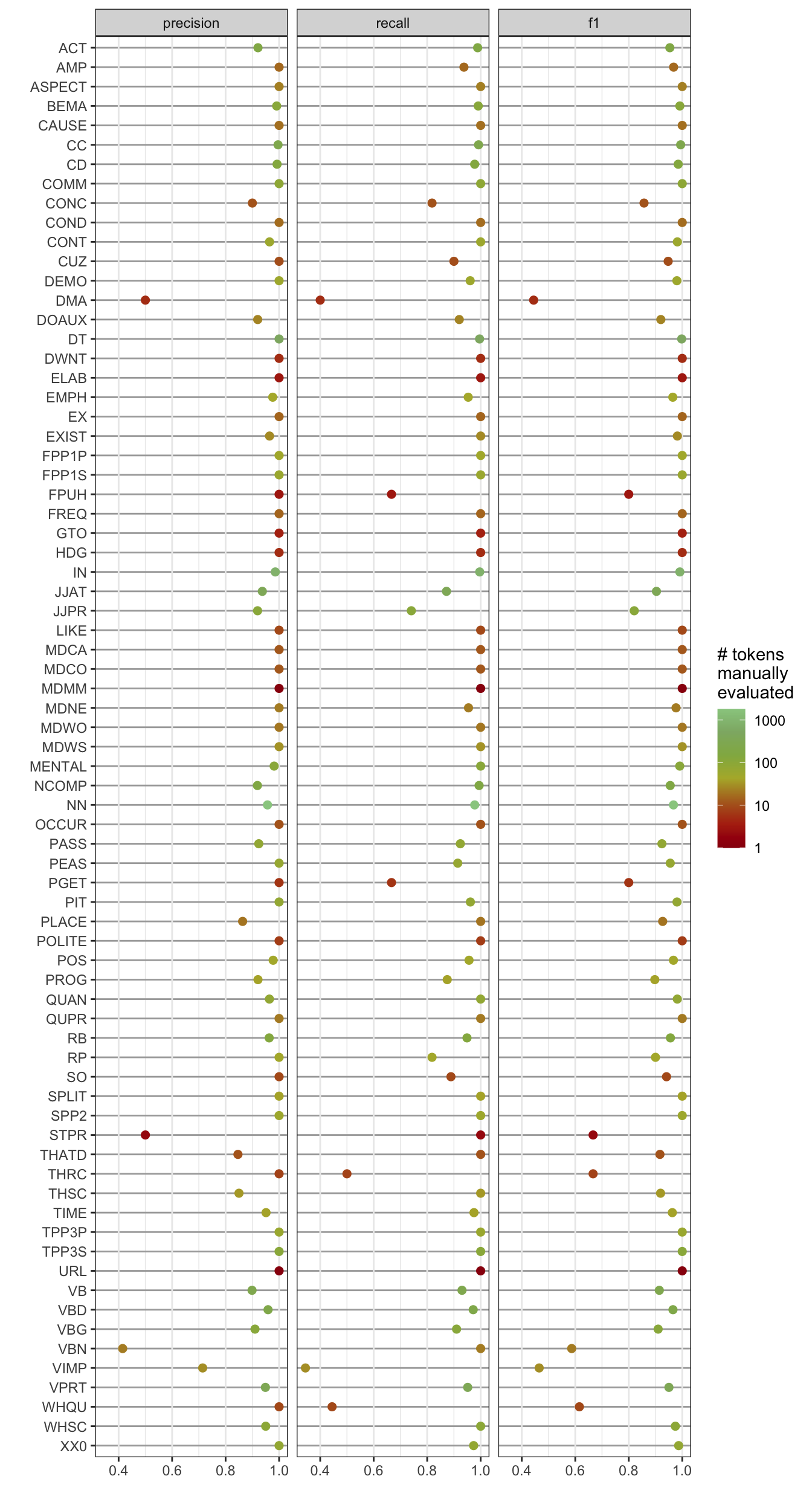
Code
#ggsave(here("plots", "TaggerAccuracyPlot.svg"), width = 7, height = 12)D.6 Exploring tagger errors
To inspect regular/systematic tagger errors, we add an error tag with the incorrectly assigned tag and underscore and then the correct “gold” label.
Code
errors <- TaggerEval |>
  filter(Evaluation=="FALSE") |>
  filter(TagGold != "UNCLEAR") |>
  mutate(Error = paste(Tag, TagGold, sep = " -> "))

FreqErrors <- errors |>
  #filter(Corpus %in% c("TEC-Fr", "TEC-Ger", "TEC-Sp")) |>
  count(Error) |>
  arrange(desc(n))

# Number of error types that only occur once
once <- FreqErrors |>
  filter(n == 1) |>
  nrow()
The total number of errors is 817. Of those, 94 occur just once. In total, there are 198 different types of errors. The most frequent 10 are:
| Error | n |
|---|---|
| NCOMP -> NULL | 37 |
| NN -> JJAT | 35 |
| JJAT -> NN | 27 |
| NN -> VB | 27 |
| IN -> RP | 25 |
| NN -> VPRT | 24 |
| VB -> NN | 22 |
| THSC -> DEMO | 19 |
| VB -> VIMP | 19 |
| NN -> OCR | 16 |
| VBN -> JJAT | 16 |
| ACT -> NULL | 15 |
| THATD -> NULL | 15 |
| CD -> NN | 12 |
| MENTAL -> NULL | 12 |
| NN -> VBG | 11 |
| NN -> VIMP | 11 |
| THSC -> THRC | 11 |
| VBG -> PROG | 11 |
| VBN -> JJPR | 11 |
The code in the following chunk can be used to take a closer look at specific types of frequent errors.
errors |>
  filter(Error == "NN -> JJAT") |>
  select(-Output, -Corpus, -Tag, -TagGold) |>
  filter(grepl(x = Token, pattern = "[A-Z]+.")) |>
kable(digits = 2)| FileID | Register | Token | Evaluation | Error |
|---|---|---|---|---|
| BNCBEFor32 | internet | Intermediate | FALSE | NN -> JJAT |
| BNCBMass16 | news | FINAL | FALSE | NN -> JJAT |
| BNCBMass16 | news | Big | FALSE | NN -> JJAT |
| BNCBReg111 | news | Scottish | FALSE | NN -> JJAT |
| BNCBReg111 | news | Scottish | FALSE | NN -> JJAT |
| BNCBReg111 | news | Mental | FALSE | NN -> JJAT |
| BNCBReg111 | news | Scottish | FALSE | NN -> JJAT |
| BNCBReg111 | news | Central | FALSE | NN -> JJAT |
| BNCBReg750 | news | English | FALSE | NN -> JJAT |
| BNCBReg750 | news | Natural | FALSE | NN -> JJAT |
| BNCBReg750 | news | European | FALSE | NN -> JJAT |
| BNCBReg750 | news | Christian | FALSE | NN -> JJAT |
| BNCBReg750 | news | Social | FALSE | NN -> JJAT |
| BNCBReg750 | news | Common | FALSE | NN -> JJAT |
| BNCBSer486 | news | Northern | FALSE | NN -> JJAT |
| BNCBSer486 | news | Northern | FALSE | NN -> JJAT |
| BNCBSer486 | news | Northern | FALSE | NN -> JJAT |
| BNCBSer562 | news | United | FALSE | NN -> JJAT |
| BNCBSer562 | news | White | FALSE | NN -> JJAT |
| BNCBSer562 | news | Untold | FALSE | NN -> JJAT |
| BNCBSer562 | news | New | FALSE | NN -> JJAT |
| SEL5 | spoken | Black | FALSE | NN -> JJAT |
errors |>
  filter(Error %in% c("NN -> VB", "VB -> NN", "NN -> VPRT", "VPRT -> NN")) |>
  count(Token) |>
  arrange(desc(n)) |>
  filter(n > 1) |>
kable(digits = 2) | Token | n |
|---|---|
| mince | 5 |
| build | 4 |
| win | 4 |
| hunt | 3 |
| wags | 3 |
| throw | 2 |
| look | 2 |
| swamp | 2 |
| stop | 2 |
| defeats | 2 |
| Token | n |
|---|---|
| win | 3 |
| throw | 2 |
| lost | 2 |
| left | 1 |
| waiting | 1 |
| working | 1 |
| running | 1 |
| done | 1 |
| fixed | 1 |
| Play | 1 |
| reached | 1 |
For more information on the MFTE evaluation, see (Le Foll 2021) and https://github.com/elenlefoll/MultiFeatureTaggerEnglish.
D.7 Packages used in this script
D.7.1 Package names and versions
R version 4.4.1 (2024-06-14)
Platform: aarch64-apple-darwin20
Running under: macOS Sonoma 14.5

Matrix products: default
BLAS:   /Library/Frameworks/R.framework/Versions/4.4-arm64/Resources/lib/libRblas.0.dylib
LAPACK: /Library/Frameworks/R.framework/Versions/4.4-arm64/Resources/lib/libRlapack.dylib;  LAPACK version 3.12.0

locale:
[1] en_US.UTF-8/en_US.UTF-8/en_US.UTF-8/C/en_US.UTF-8/en_US.UTF-8

time zone: Europe/Madrid
tzcode source: internal

attached base packages:
[1] stats     graphics  grDevices datasets  utils     methods   base

other attached packages:
 [1] knitcitations_1.0.12 lubridate_1.9.3      forcats_1.0.0
 [4] stringr_1.5.1        dplyr_1.1.4          purrr_1.0.2
 [7] readr_2.1.5          tidyr_1.3.1          tibble_3.2.1
[10] tidyverse_2.0.0      readxl_1.4.3         paletteer_1.6.0
[13] knitr_1.48           here_1.0.1           harrypotter_2.1.1
[16] caret_6.0-94         lattice_0.22-6       ggplot2_3.5.1

loaded via a namespace (and not attached):
 [1] tidyselect_1.2.1     timeDate_4032.109    fastmap_1.2.0
 [4] pROC_1.18.5          digest_0.6.36        rpart_4.1.23
 [7] timechange_0.3.0     lifecycle_1.0.4      survival_3.6-4
[10] magrittr_2.0.3       compiler_4.4.1       rlang_1.1.4
[13] tools_4.4.1          utf8_1.2.4           yaml_2.3.9
[16] data.table_1.15.4    xml2_1.3.6           plyr_1.8.9
[19] withr_3.0.0          nnet_7.3-19          grid_4.4.1
[22] stats4_4.4.1         fansi_1.0.6          colorspace_2.1-0
[25] future_1.33.2        globals_0.16.3       scales_1.3.0
[28] iterators_1.0.14     MASS_7.3-60.2        cli_3.6.3
[31] rmarkdown_2.27       generics_0.1.3       rstudioapi_0.16.0
[34] future.apply_1.11.2  httr_1.4.7           tzdb_0.4.0
[37] reshape2_1.4.4       splines_4.4.1        parallel_4.4.1
[40] BiocManager_1.30.23  cellranger_1.1.0     vctrs_0.6.5
[43] hardhat_1.4.0        Matrix_1.7-0         jsonlite_1.8.8
[46] hms_1.1.3            listenv_0.9.1        foreach_1.5.2
[49] gower_1.0.1          recipes_1.1.0        bibtex_0.5.1
[52] glue_1.7.0           parallelly_1.37.1    RefManageR_1.4.0
[55] rematch2_2.1.2       codetools_0.2-20     stringi_1.8.4
[58] gtable_0.3.5         munsell_0.5.1        pillar_1.9.0
[61] htmltools_0.5.8.1    ipred_0.9-15         lava_1.8.0
[64] R6_2.5.1             rprojroot_2.0.4      evaluate_0.24.0
[67] backports_1.5.0      renv_1.0.3           class_7.3-22
[70] Rcpp_1.0.13          gridExtra_2.3        nlme_3.1-164
[73] prodlim_2024.06.25   xfun_0.46            ModelMetrics_1.2.2.2
[76] pkgconfig_2.0.3
D.7.2 Package references
[1] S. A. file. paletteer: Comprehensive Collection of Color Palettes. R package version 1.6.0. 2024. https://github.com/EmilHvitfeldt/paletteer.
[2] G. Grolemund and H. Wickham. “Dates and Times Made Easy with lubridate”. In: Journal of Statistical Software 40.3 (2011), pp. 1-25. https://www.jstatsoft.org/v40/i03/.
[3] A. Jimenez Rico. harrypotter: Palettes Generated from All “Harry Potter” Movies. R package version 2.1.1. 2020. https://github.com/aljrico/harrypotter.
[4] M. Kuhn. caret: Classification and Regression Training. R package version 6.0-94. 2023. https://github.com/topepo/caret/.
[5] Kuhn and Max. “Building Predictive Models in R Using the caret Package”. In: Journal of Statistical Software 28.5 (2008), p. 1–26. DOI: 10.18637/jss.v028.i05. https://www.jstatsoft.org/index.php/jss/article/view/v028i05.
[6] K. Müller. here: A Simpler Way to Find Your Files. R package version 1.0.1. 2020. https://here.r-lib.org/.
[7] K. Müller and H. Wickham. tibble: Simple Data Frames. R package version 3.2.1. 2023. https://tibble.tidyverse.org/.
[8] R Core Team. R: A Language and Environment for Statistical Computing. R Foundation for Statistical Computing. Vienna, Austria, 2024. https://www.R-project.org/.
[9] D. Sarkar. Lattice: Multivariate Data Visualization with R. New York: Springer, 2008. ISBN: 978-0-387-75968-5. http://lmdvr.r-forge.r-project.org.
[10] D. Sarkar. lattice: Trellis Graphics for R. R package version 0.22-6. 2024. https://lattice.r-forge.r-project.org/.
[11] V. Spinu, G. Grolemund, and H. Wickham. lubridate: Make Dealing with Dates a Little Easier. R package version 1.9.3. 2023. https://lubridate.tidyverse.org.
[12] H. Wickham. forcats: Tools for Working with Categorical Variables (Factors). R package version 1.0.0. 2023. https://forcats.tidyverse.org/.
[13] H. Wickham. ggplot2: Elegant Graphics for Data Analysis. Springer-Verlag New York, 2016. ISBN: 978-3-319-24277-4. https://ggplot2.tidyverse.org.
[14] H. Wickham. stringr: Simple, Consistent Wrappers for Common String Operations. R package version 1.5.1. 2023. https://stringr.tidyverse.org.
[15] H. Wickham. tidyverse: Easily Install and Load the Tidyverse. R package version 2.0.0. 2023. https://tidyverse.tidyverse.org.
[16] H. Wickham, M. Averick, J. Bryan, et al. “Welcome to the tidyverse”. In: Journal of Open Source Software 4.43 (2019), p. 1686. DOI: 10.21105/joss.01686.
[17] H. Wickham and J. Bryan. readxl: Read Excel Files. R package version 1.4.3. 2023. https://readxl.tidyverse.org.
[18] H. Wickham, W. Chang, L. Henry, et al. ggplot2: Create Elegant Data Visualisations Using the Grammar of Graphics. R package version 3.5.1. 2024. https://ggplot2.tidyverse.org.
[19] H. Wickham, R. François, L. Henry, et al. dplyr: A Grammar of Data Manipulation. R package version 1.1.4. 2023. https://dplyr.tidyverse.org.
[20] H. Wickham and L. Henry. purrr: Functional Programming Tools. R package version 1.0.2. 2023. https://purrr.tidyverse.org/.
[21] H. Wickham, J. Hester, and J. Bryan. readr: Read Rectangular Text Data. R package version 2.1.5. 2024. https://readr.tidyverse.org.
[22] H. Wickham, D. Vaughan, and M. Girlich. tidyr: Tidy Messy Data. R package version 1.3.1. 2024. https://tidyr.tidyverse.org.
[23] Y. Xie. Dynamic Documents with R and knitr. 2nd. ISBN 978-1498716963. Boca Raton, Florida: Chapman and Hall/CRC, 2015. https://yihui.org/knitr/.
[24] Y. Xie. “knitr: A Comprehensive Tool for Reproducible Research in R”. In: Implementing Reproducible Computational Research. Ed. by V. Stodden, F. Leisch and R. D. Peng. ISBN 978-1466561595. Chapman and Hall/CRC, 2014.
[25] Y. Xie. knitr: A General-Purpose Package for Dynamic Report Generation in R. R package version 1.48. 2024. https://yihui.org/knitr/.