#renv::restore() # Restore the project's dependencies from the lockfile to ensure that same package versions are used as in the original study

library(caret) # For its confusion matrix function
library(cowplot)
library(DescTools) # For 95% CI
library(emmeans)
library(factoextra) # For circular graphs of variables
library(forcats) # For data manipulation
library(ggthemes) # For theme of factoextra plots
library(here) # For dynamic file paths
library(knitr) # Loaded to display the tables using the kable() function
library(lme4) # For linear regression modelling
library(patchwork) # To create figures with more than one plot
library(PCAtools) # For nice biplots of PCA results
library(psych) # For various useful stats function
library(sjPlot) # For model plots and tables
library(tidyverse) # For data wrangling
library(visreg) # For plots of interaction effects

# From https://github.com/RainCloudPlots/RainCloudPlots:
source(here("R_rainclouds.R")) # For geom_flat_violin rainplotsAppendix F — Data Analysis for the Model of Intra-Textbook Variation
This script documents the analysis of the pre-processed data from the Textbook English Corpus (TEC) to arrive at the multi-dimensional model of intra-textbook linguistic variation (Chapter 6). It generates all of the statistics and plots included in the book, as well as many others that were used in the analysis, but not included in the book for reasons of space.
F.1 Packages required
The following packages must be installed and loaded to carry out the following analyses.
F.2 Preparing the data for PCA
F.2.1 TEC data import
Code
TxBcounts <- readRDS(here("data", "processed", "TxBcounts3.rds"))
# colnames(TxBcounts)
# nrow(TxBcounts)

TxBzlogcounts <- readRDS(here("data", "processed", "TxBzlogcounts.rds"))
# nrow(TxBzlogcounts)
# colnames(TxBzlogcounts)

TxBdata <- cbind(TxBcounts[,1:6], as.data.frame(TxBzlogcounts))
# str(TxBdata)
First, the TEC data as processed in Appendix D is imported. It comprises 1,961 texts/files, each with logged standardised normalised frequencies for 66 linguistic features.
F.3 Checking the factorability of data
The overall MSA value of the dataset is 0.86. The features have the following individual MSA values (ordered from lowest to largest):
  MDWO   MDWS   MDNE   MDCA    VBD   VPRT    POS    ACT   FREQ  TPP3S     LD
  0.34   0.46   0.52   0.53   0.59   0.60   0.64   0.65   0.65   0.66   0.68
 CAUSE   COND   MDCO   VIMP  NCOMP     DT  TPP3P   STPR     RP   SPP2 MENTAL
  0.69   0.75   0.77   0.78   0.79   0.80   0.80   0.81   0.81   0.83   0.84
 DOAUX   WHSC    VBG  EXIST  THATD   COMM  FPP1S     IN     NN   WHQU   JJAT
  0.84   0.85   0.86   0.86   0.86   0.87   0.87   0.88   0.88   0.89   0.89
  DEMO   THRC ASPECT     CC     EX  OCCUR   PEAS    TTR   YNQU    AWL   QUAN
  0.89   0.89   0.90   0.90   0.90   0.90   0.91   0.91   0.91   0.92   0.92
 FPP1P   PROG    XX0   CONT   TIME   BEMA  SPLIT   PASS   JJPR    AMP   QUPR
  0.92   0.92   0.92   0.92   0.93   0.93   0.93   0.94   0.94   0.95   0.95
  THSC     RB   FPUH    CUZ    VBN    PIT    DMA POLITE   EMPH    HDG  PLACE
  0.95   0.95   0.95   0.95   0.95   0.96   0.96   0.96   0.96   0.96   0.97
F.3.1 Removal of feature with MSAs of < 0.5
We first remove the first feature with an individual MSA < 0.5, then check the MSA values again and continue removing features one by one if necessary.
The overall MSA value of the dataset is now 0.87. None of the remaining features have individual MSA values below 0.5:
MDWS MDNE MDCA VBD POS VPRT FREQ ACT TPP3S LD CAUSE
0.55 0.58 0.61 0.63 0.64 0.65 0.65 0.66 0.66 0.69 0.70
MDCO COND DT TPP3P VIMP NCOMP RP STPR SPP2 DOAUX MENTAL
0.77 0.80 0.80 0.80 0.81 0.81 0.81 0.82 0.83 0.84 0.85
VBG WHSC EXIST THATD FPP1S COMM IN NN DEMO WHQU THRC
0.85 0.85 0.86 0.87 0.87 0.87 0.88 0.89 0.89 0.89 0.89
JJAT ASPECT PEAS EX OCCUR CC TTR YNQU AWL QUAN FPP1P
0.89 0.89 0.90 0.90 0.91 0.91 0.91 0.91 0.92 0.92 0.92
TIME XX0 CONT PROG BEMA SPLIT PASS JJPR THSC AMP RB
0.92 0.92 0.93 0.93 0.93 0.93 0.94 0.94 0.95 0.95 0.95
QUPR FPUH PIT VBN DMA CUZ POLITE EMPH HDG PLACE
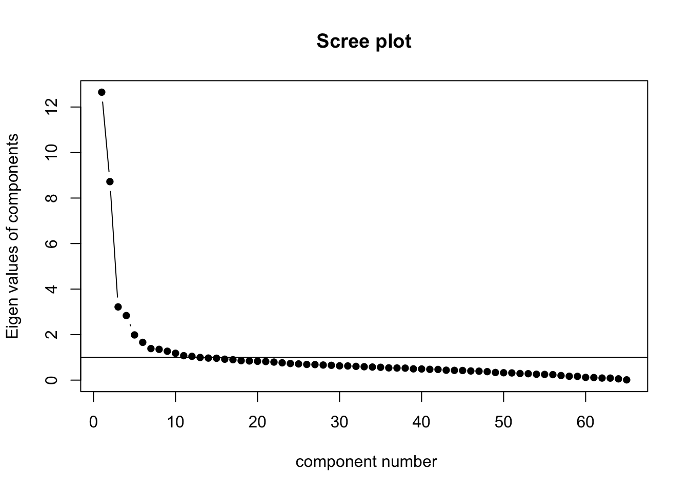
0.95 0.95 0.96 0.96 0.96 0.96 0.96 0.96 0.96 0.97 F.3.2 Choosing the number of principal components to retain
On the basis of this scree plot, six principal components were initially retained.
Code
F.3.3 Excluding features with low final communalites
We first check whether some feature have extremely low communalities (see https://rdrr.io/cran/FactorAssumptions/man/communalities_optimal_solution.html).
  STPR   MDNE    HDG  CAUSE   FREQ   THRC    POS   PROG    ACT   DEMO   MDWS
  0.09   0.17   0.17   0.19   0.22   0.22   0.24   0.26   0.26   0.27   0.28
   CUZ   COND   QUPR  EXIST   MDCO  NCOMP  OCCUR   TIME ASPECT  TPP3P    AMP
  0.28   0.28   0.29   0.29   0.31   0.31   0.32   0.32   0.33   0.33   0.34
    RP  THATD   THSC     EX  FPP1P  PLACE    PIT    VBG   PEAS   MDCA  DOAUX
  0.34   0.36   0.39   0.43   0.43   0.43   0.45   0.46   0.47   0.48   0.48
   VBN   JJPR   JJAT   WHSC  SPLIT   EMPH   QUAN MENTAL  TPP3S   PASS   YNQU
  0.48   0.49   0.49   0.50   0.51   0.53   0.55   0.56   0.56   0.57   0.58
POLITE     RB     CC    XX0     DT   COMM   WHQU    TTR  FPP1S     IN     LD
  0.58   0.58   0.58   0.59   0.62   0.62   0.64   0.65   0.67   0.68   0.68
  FPUH   VPRT   SPP2   BEMA    DMA    VBD    AWL   CONT     NN   VIMP
  0.70   0.71   0.72   0.74   0.74   0.80   0.85   0.85   0.87   0.90
As we chose to exclude features with communalities of < 0.2, we remove STPR, HDG, MDNE and CAUSE from the dataset to be analysed.
The overall MSA value of the dataset is now 0.88. None of the remaining features have individual MSA values below 0.5:
  MDWS   MDCA    POS   FREQ    VBD  TPP3S   VPRT    ACT     LD   COND     DT
  0.54   0.64   0.64   0.65   0.65   0.66   0.66   0.67   0.69   0.78   0.79
  MDCO  TPP3P     RP  NCOMP   VIMP   SPP2  DOAUX MENTAL   WHSC    VBG  THATD
  0.79   0.81   0.82   0.82   0.82   0.82   0.84   0.85   0.86   0.86   0.86
 EXIST  FPP1S   COMM     NN     IN   WHQU   DEMO ASPECT   JJAT   THRC     EX
  0.86   0.87   0.88   0.89   0.89   0.89   0.89   0.89   0.89   0.90   0.90
 OCCUR   PEAS     CC   YNQU   QUAN    AWL   TIME    XX0  FPP1P    TTR   CONT
  0.90   0.91   0.91   0.91   0.91   0.92   0.92   0.92   0.92   0.92   0.93
  PROG   BEMA  SPLIT   PASS   JJPR   THSC     RB   QUPR    AMP   FPUH    PIT
  0.93   0.93   0.93   0.94   0.94   0.95   0.95   0.95   0.95   0.95   0.95
   VBN    DMA POLITE    CUZ   EMPH  PLACE
  0.95   0.96   0.96   0.96   0.96   0.97
The final number of linguistic features entered in the intra-textbook model of linguistic variation is 61.
F.4 Testing the effect of rotating the components
This chunk was used when considering whether or not to rotate the components (see methods section). Ultimately, the components were not rotated.
# Comparing a rotated vs. a non-rotated solution

#TxBdata <- readRDS(here("data", "processed", "TxBdataforPCA.rds"))

# No rotation
pca2 <- psych::principal(TxBdata[,7:ncol(TxBdata)],
                         nfactors = 6,
                         rotate = "none")

pca2$loadings

biplot.psych(pca2,
             vars = TRUE,
             choose=c(1,2),
             )

# Promax rotation
pca2.rotated <- psych::principal(TxBdata[,7:ncol(TxBdata)],
                         nfactors = 6,
                         rotate = "promax")

# This summary shows the component correlations which is particularly interesting
pca2.rotated

pca2.rotated$loadings

biplot.psych(pca2.rotated, vars = TRUE, choose=c(1,2))
F.5 Principal Component Analysis (PCA)
F.5.1 Using the full dataset
Except outliers removed as part of the data preparation (see Appendix D).
F.5.2 Using random subsets of the data
Alternatively, it is possible to conduct the PCA on random subsets of the data to test the stability of the solution. Re-running this line will generate a new subset of the TEC texts containing 2/3 of the texts randomly sampled.
TxBdata <- readRDS(here("data", "processed", "TxBdataforPCA.rds")) |>
  slice_sample(n = round(1961*0.6), replace = FALSE)

nrow(TxBdata)
TxBdata$Filename[1:10]
nrow(TxBdata) / (ncol(TxBdata)-6) # Check that there is enough data to conduct a PCA. This ratio should be at least 5 (see Friginal & Hardy 2014: 303–304).
F.5.3 Using specific subsets of the data
The following chunk can be used to perform the PCA on a country subset of the data to test the stability of the solution. See (Le Foll) for a detailed analysis of the subcorpus of textbooks used in Germany.
TxBdata <- readRDS(here("data", "processed", "TxBdataforPCA.rds")) |>
  #filter(Country == "France")
  #filter(Country == "Germany")
  filter(Country == "Spain")

nrow(TxBdata)
TxBdata$Filename[1:10] # Check data
nrow(TxBdata) / (ncol(TxBdata)-6) # Check that there is enough data to conduct a PCA. This should be > 5 (see Friginal & Hardy 2014: 303–304).
F.5.4 Performing the PCA
We perform the PCA using the prcomp function and print a summary of the results.
Code
Importance of first k=6 (out of 61) components:
                          PC1    PC2     PC3     PC4     PC5     PC6
Standard deviation     2.1693 1.7776 1.08902 1.00207 0.84288 0.76792
Proportion of Variance 0.2108 0.1416 0.05313 0.04499 0.03183 0.02642
Cumulative Proportion  0.2108 0.3524 0.40553 0.45051 0.48234 0.50876
F.6 Plotting PCA results
F.6.1 3D plots
The following chunk can be used to create projections of TEC texts on three dimensions of the model. These plots cannot be rendered in two dimensions and are therefore not generated in the present document. For more information on the pca3d library, see: https://cran.r-project.org/web/packages/pca3d/vignettes/pca3d.pdf.
library(pca3d) # For 3-D plots

col <- palette[c(1:3,8,7)] # without poetry
names(col) <- c("Conversation", "Fiction", "Informative", "Instructional", "Personal")
scales::show_col(col) # Check colours

pca3d(pca,
      group = register,
      components = 1:3,
      #components = 4:6,
      show.ellipses=FALSE,
      ellipse.ci=0.75,
      show.plane=FALSE,
      col = col,
      shape = "sphere",
      radius = 1,
      legend = "right")

snapshotPCA3d(here("plots", "PCA_TxB_3Dsnapshot.png"))

names(col) <- c("C", "B", "E", "A", "D") # To colour the dots according to the profiency level of the textbooks
pca3d(pca,
      components = 4:6,
      group = level,
      show.ellipses=FALSE,
      ellipse.ci=0.75,
      show.plane=FALSE,
      col = col,
      shape = "sphere",
      radius = 0.8,
      legend = "right")
F.7 Two-dimensional plots (biplots)
These plots were generated using the PCAtools package, which requires the data to be formatted in a rather unconventional way so it needs to wrangled first.
F.7.1 Data wrangling for PCAtools
Code
#TxBdata <- readRDS(here("data", "processed", "TxBdataforPCA.rds"))

TxBdata2meta <- TxBdata[,1:6]
rownames(TxBdata2meta) <- TxBdata2meta$Filename
TxBdata2meta <- TxBdata2meta |> select(-Filename)
#head(TxBdata2meta)

TxBdata2 = TxBdata
rownames(TxBdata2) <- TxBdata2$Filename
TxBdata2num <- as.data.frame(base::t(TxBdata2[,7:ncol(TxBdata2)]))
#TxBdata2num[1:12,1:3] # Check sanity of data

p <- PCAtools::pca(TxBdata2num,
         metadata = TxBdata2meta,
         scale = FALSE)
F.7.2 Pairs plot
We first produce a scatterplot matrix of all the combinations of the first six dimensions of the model of intra-textbook variation. Note that the number before the comma on each axis label shows which principal component is plotted on that axis; this is followed by the percentage of the total variance explained by that particular component. The colours correspond to the text registers.
Code
## Colour and shape scheme for all biplots
colkey = c(Conversation="#BD241E", Fiction="#A18A33", Informative="#15274D", Instructional="#F9B921", Personal="#722672")
shapekey = c(A=1, B=2, C=6, D=0, E=5)

## Very slow, open in zoomed out window!
# Add legend manually? Yes (take it from the biplot code below), sadly really the simplest solution, here. Or use Evert's mvar.pairs plot function (though that also requires manual axis annotation).

# png(here("plots", "PCA_TxB_pairsplot.png"), width = 12, height= 19, units = "cm", res = 300)
PCAtools::pairsplot(p,
                 triangle = FALSE,
                 components = 1:6,
                 ncol = 3,
                 nrow = 5,
                 pointSize = 0.8,
                 lab = NULL, # Otherwise will try to label each data point!
                 colby = "Register",
                 colkey = colkey,
                 shape = "Level",
                 shapekey = shapekey,
                 margingaps = unit(c(0.2, 0.2, 0.2, 0.2), "cm"),
                 legendPosition = "none")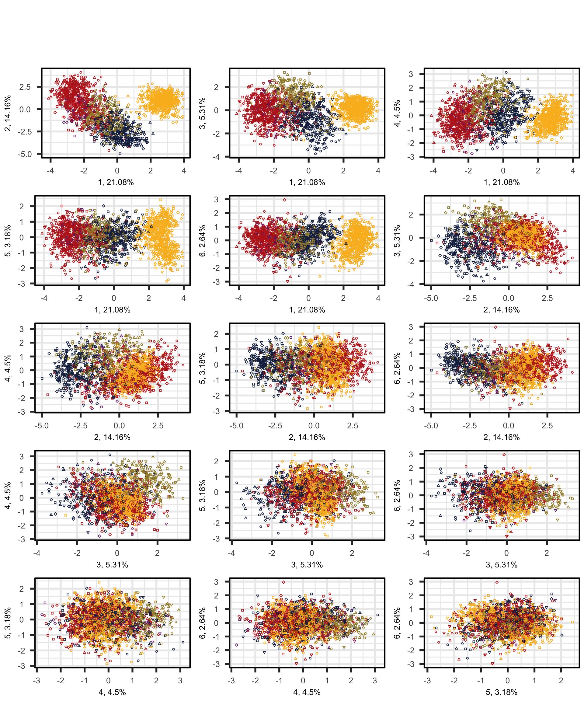
F.7.3 Bi-plots
Then, biplots of the most important dimensions are generated to examine components more carefully.
The following biplot displays the distribution of the texts of the TEC along the first and second dimensions of the intra-textbook model.
Code
colkey = c(Conversation="#BD241E", Fiction="#A18A33", Informative="#15274D", Instructional="#F9B921", Personal="#722672")
shapekey = c(A=1, B=2, C=6, D=0, E=5)

#png(here("plots", "PCA_TxB_Biplot_PC1_PC2.png"), width = 40, height= 25, units = "cm", res = 300)
PCAtools::biplot(p,
                 x = "PC1",
                 y = "PC2",
                 lab = NULL, # Otherwise will try to label each data point!
                 #xlim = c(min(p$rotated$PC1)-0.5, max(p$rotated$PC1)+0.5),
                 #ylim = c(min(p$rotated$PC2)-0.5, max(p$rotated$PC2)+0.5),
                 colby = "Register",
                 pointSize = 2,
                 colkey = colkey,
                 shape = "Level",
                 shapekey = shapekey,
                 showLoadings = FALSE,
                 ellipse = TRUE,
                 axisLabSize = 22,
                 legendPosition = 'right',
                 legendTitleSize = 22,
                 legendLabSize = 18,
                 legendIconSize = 7) +
  theme(plot.margin = unit(c(0,0,0,0.2), "cm"))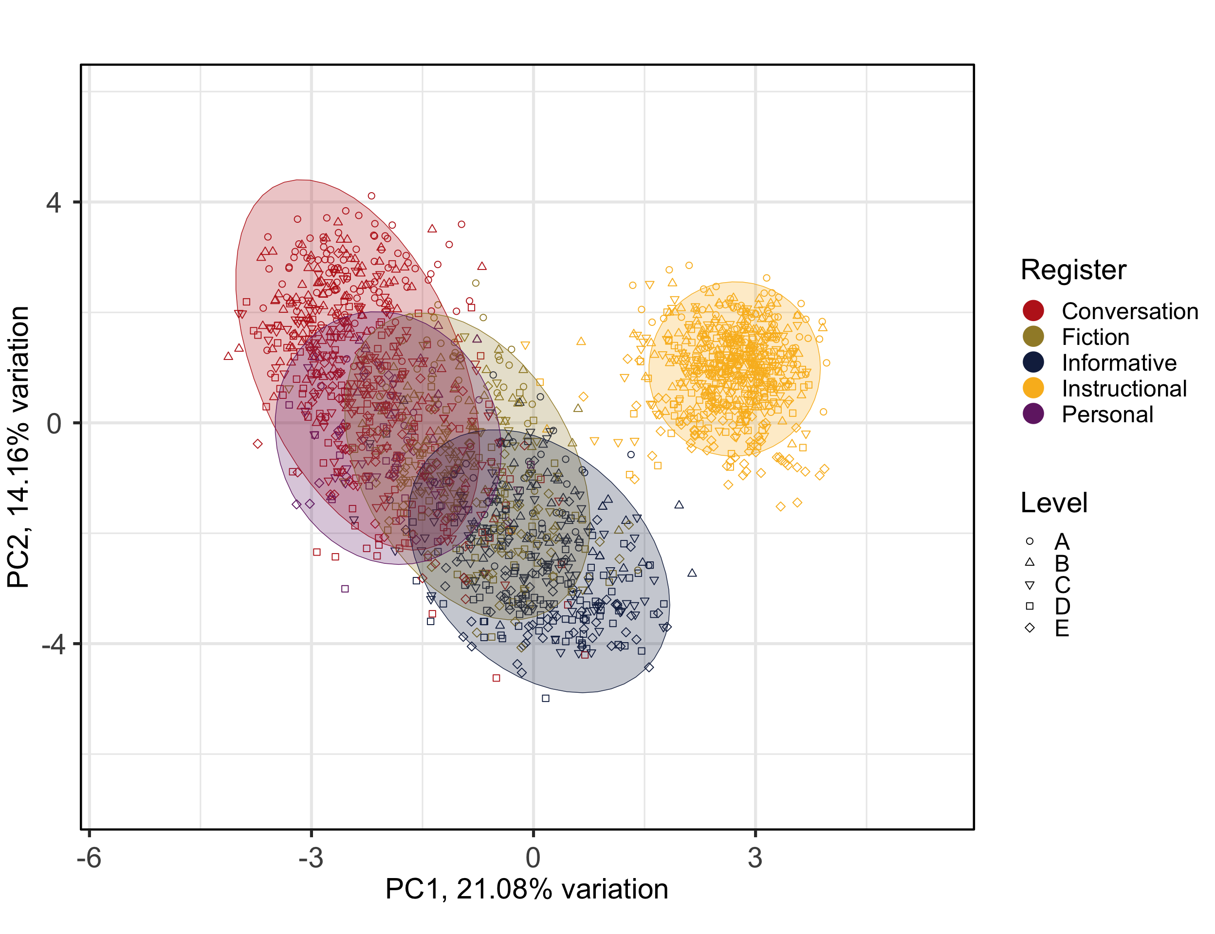
Code
#dev.off()
#ggsave(here("plots", "PCA_TxB_BiplotPC1_PC2.svg"), width = 12, height = 10)
The following code chunk can be used for the interactive examination of individual data points (i.e., texts).
library(plotly)
plot <- PCAtools::biplot(p,
x = "PC1",
y = "PC2",
lab = NULL, # Otherwise will try to label each data point!
colby = "Register",
pointSize = 2,
colkey = colkey,
shape = "Level",
shapekey = shapekey,
showLoadings = FALSE,
ellipse = TRUE,
axisLabSize = 22,
legendPosition = 'right',
legendTitleSize = 22,
legendLabSize = 18,
legendIconSize = 7) +
theme(plot.margin = unit(c(0,0,0,0.2), "cm"))
ggplotly(plot) # tooltip
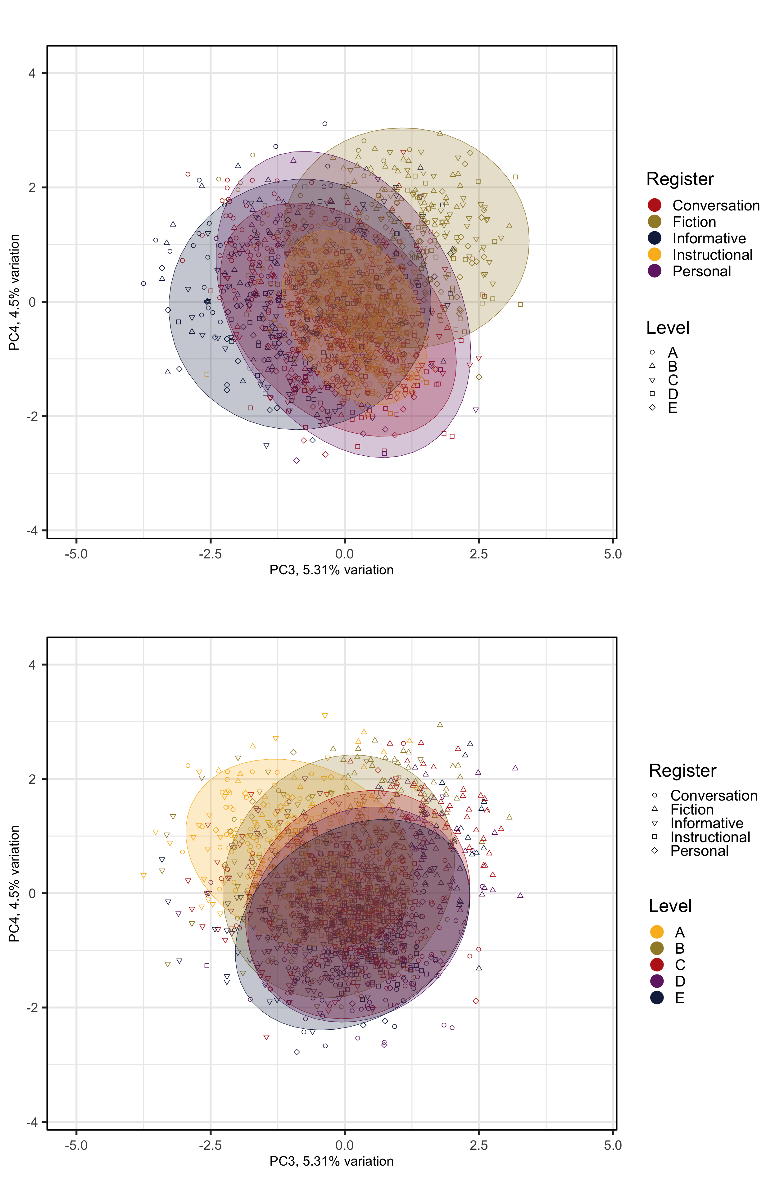
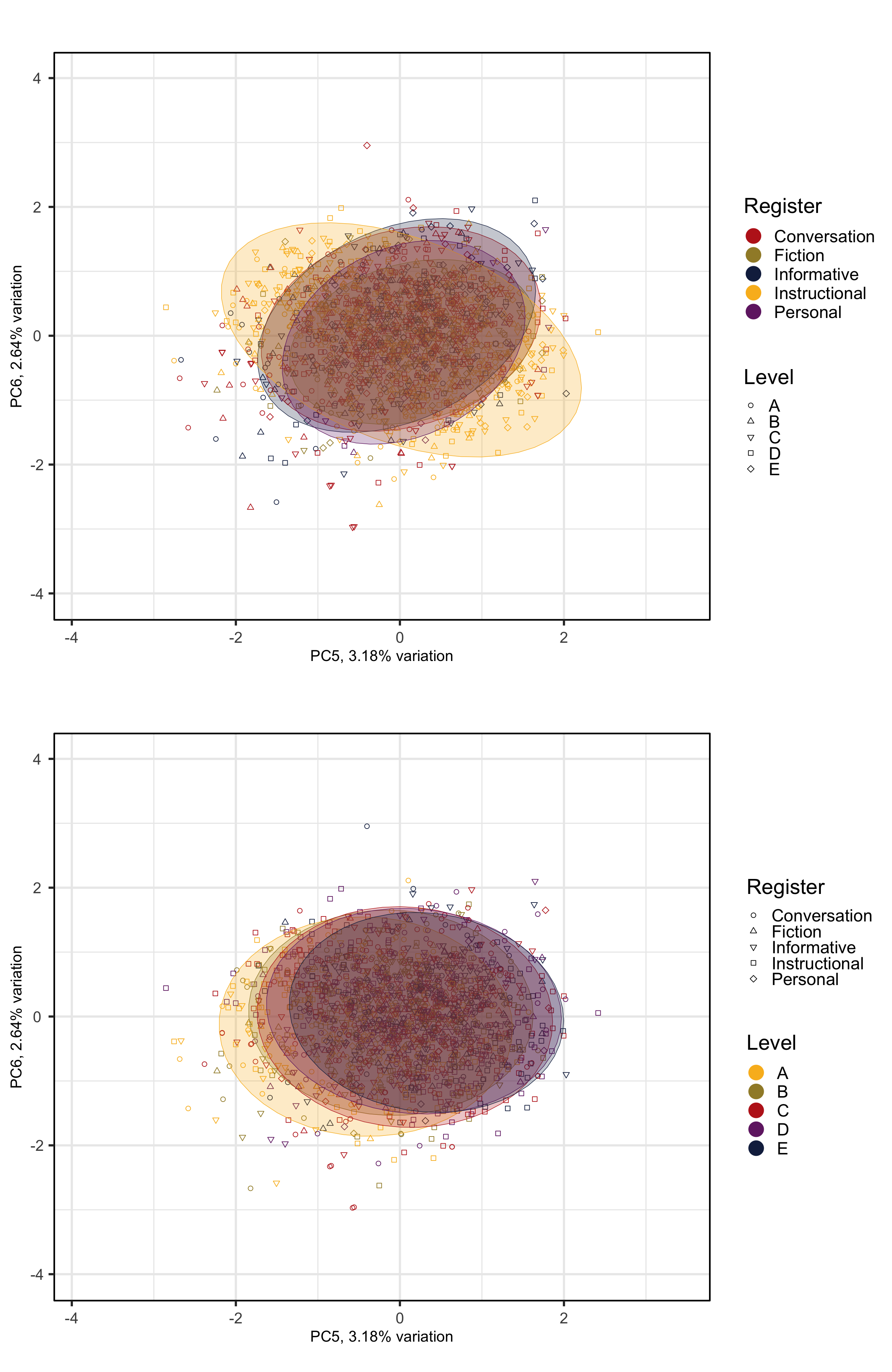
###For the fourth to sixth dimensions of the model, it is worth comparing the effet of text register with that of textbook proficiency level. Hence, the following two chunks generate biplots with colour and ellipses representing a) text register (as above) and b) textbook level (A = first year of EFL tuition at secondary school, E = fifth year).
Code
pRegisters <- PCAtools::biplot(p,
                 x = "PC3",
                 y = "PC4",
                 lab = NULL, # Otherwise will try to label each data point!
                 colby = "Register",
                 pointSize = 2,
                 colkey = colkey,
                 shape = "Level",
                 shapekey = shapekey,
                 showLoadings = FALSE,
                 ellipse = TRUE,
                 legendPosition = 'right',
                 legendTitleSize = 22,
                 legendLabSize = 18,
                 legendIconSize = 7) +
  theme(plot.margin = unit(c(0,0,0,0.2), "cm"))

#ggsave(here("plots", "PCA_TxB_BiplotPC3_PC4.svg"), width = 12, height = 10)

pRegisters2 <- PCAtools::biplot(p,
                 x = "PC5",
                 y = "PC6",
                 lab = NULL, # Otherwise will try to label each data point!
                 colby = "Register",
                 pointSize = 2,
                 colkey = colkey,
                 shape = "Level",
                 shapekey = shapekey,
                 showLoadings = FALSE,
                 ellipse = TRUE,
                 legendPosition = 'right',
                 legendTitleSize = 22,
                 legendLabSize = 18,
                 legendIconSize = 7) +
  theme(plot.margin = unit(c(0,0,0,0.2), "cm"))

#ggsave(here("plots", "PCA_TxB_BiplotPC5_PC6.svg"), width = 12, height = 10)
Code
# Inverted keys for the biplots with ellipses for Level rather than Register
colkeyLevels = c(A="#F9B921", B="#A18A33", C="#BD241E", D="#722672", E="#15274D")
shapekeyLevels = c(Conversation=1, Fiction=2, Informative=6, Instructional=0, Personal=5)

pLevels <- PCAtools::biplot(p,
                 x = "PC3",
                 y = "PC4",
                 lab = NULL, # Otherwise will try to label each data point!
                 #xlim = c(min(p$rotated$PC1)-0.5, max(p$rotated$PC1)+0.5),
                 #ylim = c(min(p$rotated$PC2)-0.5, max(p$rotated$PC2)+0.5),
                 colby = "Level",
                 pointSize = 2,
                 colkey = colkeyLevels,
                 shape = "Register",
                 shapekey = shapekeyLevels,
                 showLoadings = FALSE,
                 ellipse = TRUE,
                 legendPosition = 'right',
                 legendTitleSize = 22,
                 legendLabSize = 18,
                 legendIconSize = 7) +
  theme(plot.margin = unit(c(0,0,0,0.2), "cm"))
#ggsave(here("plots", "PCA_TxB_BiplotPC3_PC4_Level.svg"), width = 12, height = 10)

pLevels2 <- PCAtools::biplot(p,
                 x = "PC5",
                 y = "PC6",
                 lab = NULL, # Otherwise will try to label each data point!
                 #xlim = c(min(p$rotated$PC1)-0.5, max(p$rotated$PC1)+0.5),
                 #ylim = c(min(p$rotated$PC2)-0.5, max(p$rotated$PC2)+0.5),
                 colby = "Level",
                 pointSize = 2,
                 colkey = colkeyLevels,
                 shape = "Register",
                 shapekey = shapekeyLevels,
                 showLoadings = FALSE,
                 ellipse = TRUE,
                 legendPosition = 'right',
                 legendTitleSize = 22,
                 legendLabSize = 18,
                 legendIconSize = 7) +
  theme(plot.margin = unit(c(0,0,0,0.2), "cm"))
#ggsave(here("plots", "PCA_TxB_BiplotPC5_PC6_Level.svg"), width = 12, height = 10)
The following biplots display the distribution of the texts of the TEC along the third and fourth dimensions of the intra-textbook model.
The following biplots display the distribution of the texts of the TEC along the fifth and sixth dimensions of the intra-textbook model.
F.8 Feature contributions (loadings) on each component
Code
#TxBdata <- readRDS(here("data", "processed", "TxBdataforPCA.rds"))

pca <- prcomp(TxBdata[,7:ncol(TxBdata)], scale.=FALSE) # All quantitative variables for all TEC files

# The rotated data that represents the observations / samples is stored in rotated, while the variable loadings are stored in loadings
loadings <- as.data.frame(pca$rotation[,1:4])
loadings |>
  round(2) |>
kable()| PC1 | PC2 | PC3 | PC4 | |
|---|---|---|---|---|
| ACT | 0.08 | -0.11 | 0.04 | -0.10 |
| AMP | -0.12 | -0.10 | -0.11 | 0.01 |
| ASPECT | 0.10 | -0.05 | 0.14 | -0.01 |
| AWL | 0.22 | -0.16 | -0.12 | -0.13 |
| BEMA | -0.22 | 0.01 | -0.21 | 0.02 |
| CC | 0.05 | -0.21 | -0.19 | 0.00 |
| COMM | 0.20 | 0.09 | 0.14 | -0.04 |
| COND | -0.01 | -0.02 | 0.11 | -0.24 |
| CONT | -0.25 | 0.11 | -0.03 | -0.06 |
| CUZ | -0.09 | -0.13 | -0.06 | -0.02 |
| DEMO | -0.12 | 0.08 | 0.03 | -0.09 |
| DMA | -0.20 | 0.14 | -0.02 | 0.00 |
| DOAUX | -0.01 | 0.20 | 0.05 | -0.15 |
| DT | 0.12 | 0.00 | 0.31 | -0.02 |
| EMPH | -0.19 | -0.02 | 0.06 | -0.14 |
| EX | -0.10 | -0.05 | -0.11 | 0.05 |
| EXIST | -0.02 | -0.15 | -0.09 | -0.09 |
| FPP1P | -0.17 | 0.01 | -0.07 | 0.00 |
| FPP1S | -0.23 | 0.07 | 0.08 | -0.01 |
| FPUH | -0.16 | 0.15 | -0.09 | 0.07 |
| FREQ | -0.03 | -0.05 | 0.01 | -0.10 |
| IN | 0.17 | -0.18 | 0.02 | -0.08 |
| JJAT | -0.06 | -0.18 | 0.04 | -0.21 |
| JJPR | -0.17 | -0.06 | -0.11 | -0.11 |
| LD | 0.16 | -0.03 | -0.26 | -0.01 |
| MDCA | -0.04 | 0.10 | -0.18 | -0.09 |
| MDCO | -0.05 | -0.10 | 0.22 | 0.01 |
| MDWS | -0.07 | -0.01 | 0.05 | -0.16 |
| MENTAL | 0.14 | 0.13 | 0.12 | -0.25 |
| NCOMP | 0.04 | -0.05 | -0.24 | -0.15 |
| NN | 0.20 | -0.09 | -0.29 | 0.11 |
| OCCUR | 0.02 | -0.18 | 0.03 | 0.02 |
| PASS | -0.01 | -0.22 | -0.06 | -0.05 |
| PEAS | -0.06 | -0.17 | 0.13 | -0.13 |
| PIT | -0.19 | -0.04 | -0.06 | -0.06 |
| PLACE | -0.16 | -0.01 | -0.07 | 0.09 |
| POLITE | -0.14 | 0.13 | -0.07 | 0.02 |
| POS | -0.01 | 0.03 | -0.04 | 0.16 |
| PROG | -0.11 | -0.02 | 0.11 | 0.00 |
| QUAN | -0.15 | -0.03 | 0.12 | -0.19 |
| QUPR | -0.10 | -0.05 | 0.16 | -0.11 |
| RB | -0.19 | -0.08 | 0.20 | 0.00 |
| RP | 0.00 | -0.09 | 0.14 | 0.02 |
| SPLIT | -0.11 | -0.18 | 0.02 | -0.16 |
| SPP2 | 0.10 | 0.22 | -0.01 | -0.25 |
| THATD | -0.05 | 0.04 | 0.16 | -0.24 |
| THRC | 0.02 | -0.11 | -0.02 | -0.18 |
| THSC | -0.06 | -0.17 | 0.07 | -0.14 |
| TIME | -0.12 | -0.08 | -0.01 | 0.06 |
| TPP3P | -0.01 | -0.16 | -0.09 | -0.02 |
| TPP3S | -0.06 | -0.11 | 0.13 | 0.30 |
| TTR | -0.04 | -0.26 | -0.05 | -0.01 |
| VBD | -0.08 | -0.20 | 0.23 | 0.30 |
| VBG | 0.04 | -0.18 | 0.00 | -0.22 |
| VBN | 0.03 | -0.18 | -0.07 | -0.04 |
| VIMP | 0.25 | 0.15 | 0.04 | -0.08 |
| VPRT | -0.15 | 0.05 | -0.32 | -0.22 |
| WHQU | 0.11 | 0.23 | 0.00 | -0.09 |
| WHSC | 0.11 | -0.11 | 0.03 | -0.15 |
| XX0 | -0.22 | 0.03 | 0.06 | -0.06 |
| YNQU | -0.03 | 0.23 | 0.00 | -0.08 |
We can go back to the normalised frequencies of the individual features to compare them across different registers and levels, e.g.:
TxBcounts |>
  group_by(Register, Level) |>
  summarise(median(NCOMP), MAD(NCOMP)) |>
  select(1:4) |>
kable(digits=2)| Register | Level | median(NCOMP) | MAD(NCOMP) |
|---|---|---|---|
| Conversation | A | 5.69 | 2.79 |
| Conversation | B | 5.48 | 2.66 |
| Conversation | C | 5.32 | 2.58 |
| Conversation | D | 6.18 | 2.91 |
| Conversation | E | 6.21 | 2.62 |
| Fiction | A | 4.14 | 2.34 |
| Fiction | B | 3.96 | 2.17 |
| Fiction | C | 4.05 | 1.86 |
| Fiction | D | 5.05 | 2.34 |
| Fiction | E | 5.05 | 2.16 |
| Informative | A | 8.07 | 2.48 |
| Informative | B | 7.62 | 2.40 |
| Informative | C | 7.49 | 3.16 |
| Informative | D | 7.56 | 2.46 |
| Informative | E | 8.77 | 2.45 |
| Instructional | A | 6.84 | 2.54 |
| Instructional | B | 6.80 | 2.65 |
| Instructional | C | 6.14 | 2.35 |
| Instructional | D | 6.22 | 2.29 |
| Instructional | E | 6.75 | 2.69 |
| Personal | A | 6.72 | 1.42 |
| Personal | B | 4.92 | 2.33 |
| Personal | C | 5.75 | 1.45 |
| Personal | D | 6.46 | 3.19 |
| Personal | E | 8.22 | 3.09 |
Graphs of features display the features with the strongest contributions to any two dimensions of the model of intra-textbook variation. They are created using the factoextra::fviz_pca_var function.
Code
factoextra::fviz_pca_var(pca,
             axes = c(1,2),
             select.var = list(cos2 = 0.1),
             col.var = "contrib", # Colour by contributions to the PC
             gradient.cols = c("#F9B921", "#DB241E", "#722672"),
             title = "",
             repel = TRUE, # Try to avoid too much text overlapping
             ggtheme = ggthemes::theme_few())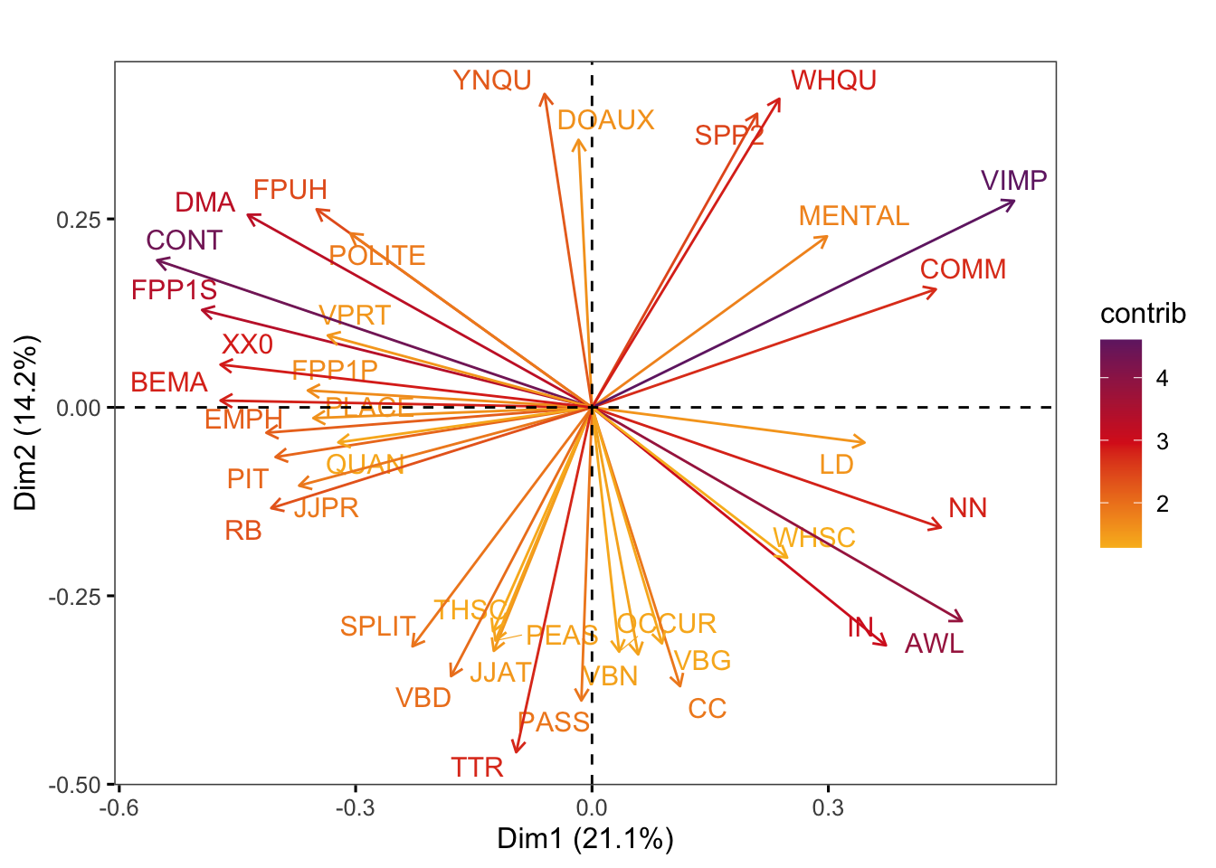
Code
#ggsave(here("plots", "fviz_pca_var_PC1_PC2.svg"), width = 11, height = 9)

factoextra::fviz_pca_var(pca,
             axes = c(3,2),
             select.var = list(contrib = 30),
             col.var = "contrib", # Colour by contributions to the PC
             gradient.cols = c("#F9B921", "#DB241E", "#722672"),
             title = "",
             repel = TRUE, # Try to avoid too much text overlapping
             ggtheme = ggthemes::theme_few())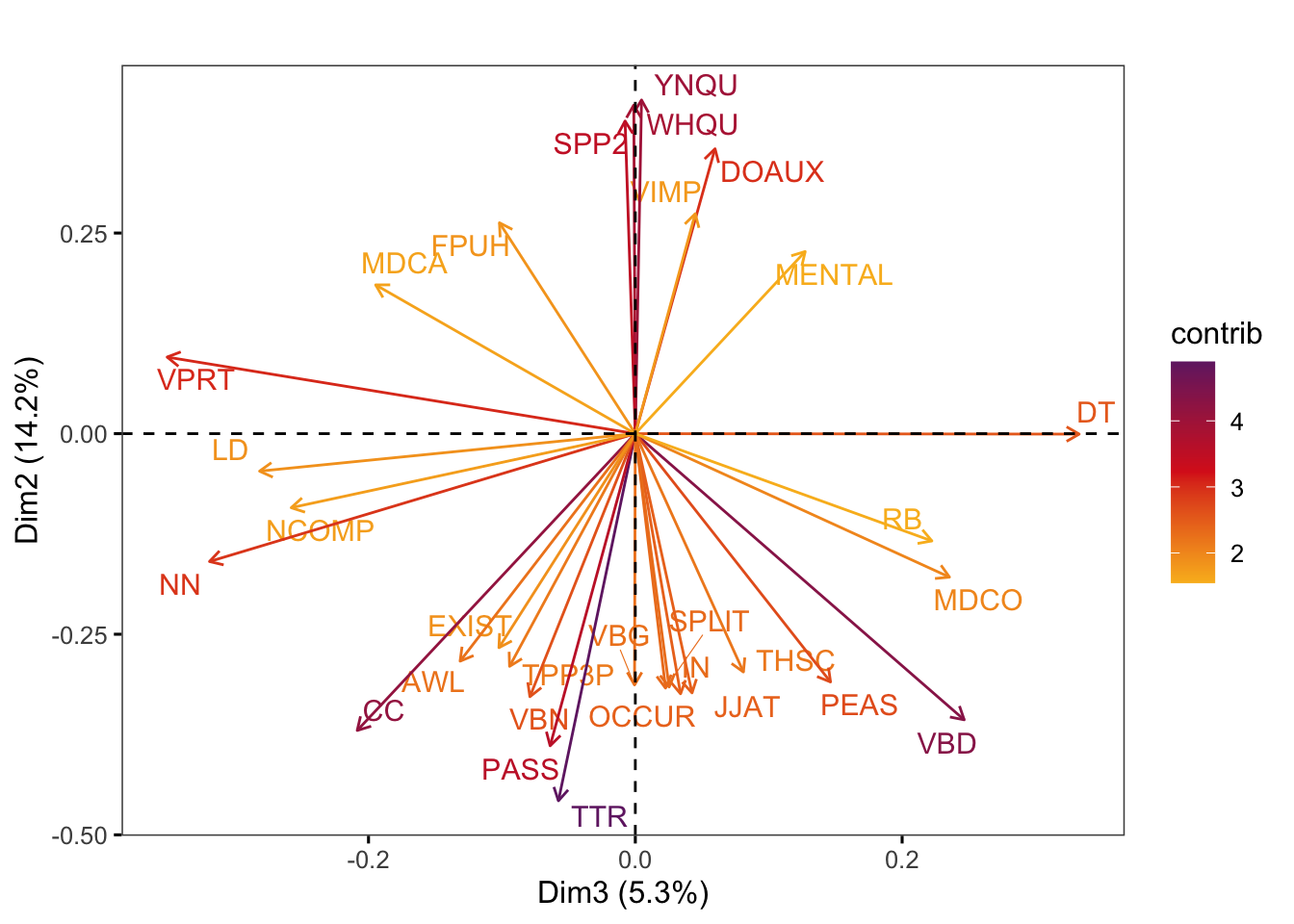
Code
#ggsave(here("plots", "fviz_pca_var_PC3_PC2.svg"), width = 9, height = 8)

factoextra::fviz_pca_var(pca,
             axes = c(3,4),
             select.var = list(contrib = 30),
             col.var = "contrib", # Colour by contributions to the PC
             gradient.cols = c("#F9B921", "#DB241E", "#722672"),
             title = "",
             repel = TRUE, # Try to avoid too much text overlapping
             ggtheme = ggthemes::theme_few())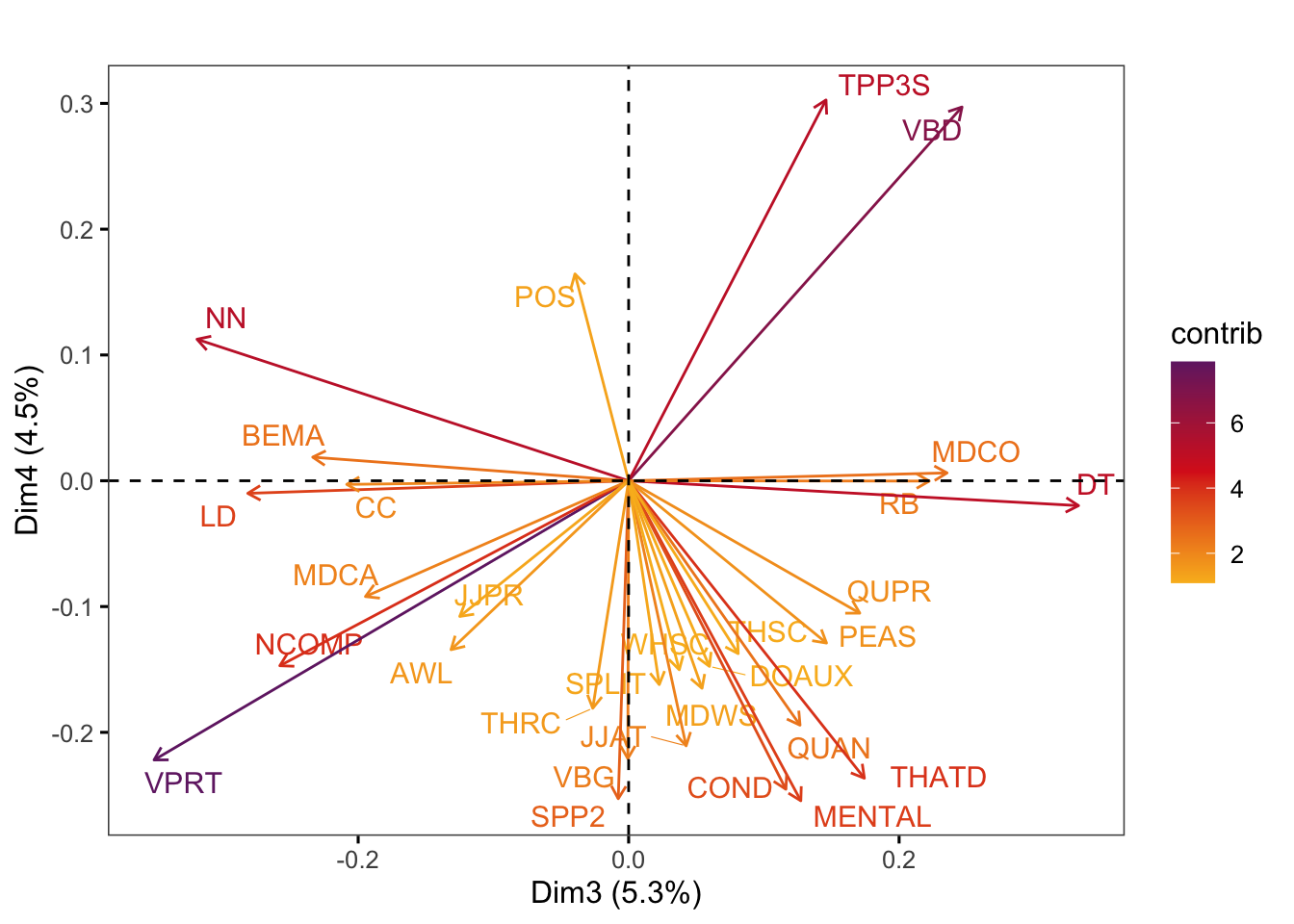
Code
#ggsave(here("plots", "fviz_pca_var_PC3_PC4.svg"), width = 9, height = 8)F.9 Exploring the dimensions of the model
We begin with some descriptive statistics of the dimension scores.
Code
# http://www.sthda.com/english/articles/31-principal-component-methods-in-r-practical-guide/118-principal-component-analysis-in-r-prcomp-vs-princomp/#pca-results-for-variables

#TxBdata <- readRDS(here("data", "processed", "TxBdataforPCA.rds"))

pca <- prcomp(TxBdata[,7:ncol(TxBdata)], scale.=FALSE) # All quantitative variables for all TxB files
register  <- factor(TxBdata[,"Register"]) # Register
level <- factor(TxBdata[,"Level"]) # Textbook proficiency level

# summary(register)
# summary(level)
# summary(pca)

## Access to the PCA results for individual PC
#pca$rotation[,1]

res.ind <- cbind(TxBdata[,1:5], as.data.frame(pca$x)[,1:6])

res.ind |>
  group_by(Register) |>
  summarise_if(is.numeric, mean) |>
kable(digits = 2)| Register | PC1 | PC2 | PC3 | PC4 | PC5 | PC6 |
|---|---|---|---|---|---|---|
| Conversation | -2.29 | 0.93 | -0.14 | -0.27 | -0.02 | 0.06 |
| Fiction | -0.85 | -0.81 | 1.02 | 1.09 | 0.11 | -0.10 |
| Informative | 0.06 | -2.45 | -0.83 | 0.01 | -0.08 | 0.12 |
| Instructional | 2.68 | 0.93 | 0.15 | -0.24 | 0.01 | -0.07 |
| Personal | -1.92 | -0.29 | -0.05 | -0.02 | 0.07 | -0.09 |
Code
res.ind |>
  group_by(Register, Level) |>
  summarise_if(is.numeric, mean) |>
kable(digits = 2)| Register | Level | PC1 | PC2 | PC3 | PC4 | PC5 | PC6 |
|---|---|---|---|---|---|---|---|
| Conversation | A | -2.39 | 2.39 | -1.23 | 0.71 | -0.45 | -0.01 |
| Conversation | B | -2.54 | 1.72 | -0.25 | 0.04 | -0.14 | 0.13 |
| Conversation | C | -2.25 | 0.70 | 0.18 | -0.41 | 0.09 | -0.02 |
| Conversation | D | -2.10 | -0.08 | 0.28 | -0.73 | 0.17 | 0.09 |
| Conversation | E | -2.13 | -0.14 | 0.07 | -0.98 | 0.16 | 0.17 |
| Fiction | A | -0.95 | 0.85 | -0.54 | 1.48 | -0.31 | -0.46 |
| Fiction | B | -0.89 | -0.14 | 0.95 | 1.78 | -0.06 | -0.03 |
| Fiction | C | -0.98 | -0.81 | 1.62 | 1.23 | 0.26 | -0.16 |
| Fiction | D | -0.71 | -1.57 | 1.27 | 0.72 | 0.21 | -0.01 |
| Fiction | E | -0.80 | -1.45 | 1.16 | 0.56 | 0.25 | -0.01 |
| Informative | A | -0.09 | -1.11 | -1.94 | 0.87 | -0.88 | -0.15 |
| Informative | B | 0.15 | -1.67 | -1.19 | 0.46 | -0.38 | 0.13 |
| Informative | C | -0.02 | -2.37 | -0.68 | -0.03 | -0.06 | -0.01 |
| Informative | D | 0.06 | -2.89 | -0.45 | -0.19 | 0.06 | 0.10 |
| Informative | E | 0.15 | -3.13 | -0.79 | -0.38 | 0.30 | 0.43 |
| Instructional | A | 2.89 | 1.55 | -0.20 | 0.46 | -0.34 | -0.24 |
| Instructional | B | 2.68 | 1.27 | 0.09 | 0.00 | -0.12 | -0.12 |
| Instructional | C | 2.59 | 0.99 | 0.28 | -0.32 | -0.07 | 0.01 |
| Instructional | D | 2.63 | 0.70 | 0.28 | -0.49 | 0.12 | 0.07 |
| Instructional | E | 2.64 | 0.09 | 0.20 | -0.80 | 0.49 | -0.16 |
| Personal | A | -1.84 | 0.53 | -1.11 | 1.21 | -0.31 | 0.12 |
| Personal | B | -1.85 | 0.40 | -0.58 | 0.59 | 0.21 | -0.07 |
| Personal | C | -2.05 | -0.46 | 0.52 | -0.17 | 0.06 | -0.03 |
| Personal | D | -1.89 | -1.05 | 0.45 | -0.63 | 0.39 | -0.06 |
| Personal | E | -1.96 | -0.92 | 0.21 | -1.10 | -0.19 | -0.45 |
The following chunk can be used to search for example texts that are located in specific areas of the biplots. For example, we can search for texts that have high scores on Dim3 and low ones on Dim2 to proceed with a qualitative comparison and analysis of these texts.
| Filename | PC2 | PC3 |
|---|---|---|
| Achievers_B1_plus_Narrative_0005.txt | -3.88 | 2.60 |
| Solutions_Intermediate_Plus_Spoken_0018.txt | -2.08 | 2.56 |
| JTT_3_Narrative_0005.txt | -2.85 | 2.76 |
| Achievers_B2_Narrative_00031.txt | -2.61 | 2.59 |
| Access_4_Narrative_0006.txt | -2.19 | 3.18 |
F.10 Computing mixed-effects models of the dimension scores
F.10.1 Dimension 1: ‘Overt instructions and explanations’
Having compared various models, the following model is chosen as the best-fitting one.
# Models with Textbook series as random intercepts
md1 <- lmer(PC1 ~ Register*Level + (1|Series), data = res.ind, REML = FALSE)
md1Register <- lmer(PC1 ~ Register + (1|Series), data = res.ind, REML = FALSE)
md1Level <- lmer(PC1 ~ Level + (1|Series), data = res.ind, REML = FALSE)

anova(md1, md1Register, md1Level)
Data: res.ind
Models:
md1Register: PC1 ~ Register + (1 | Series)
md1Level: PC1 ~ Level + (1 | Series)
md1: PC1 ~ Register * Level + (1 | Series)
npar AIC BIC logLik deviance Chisq Df Pr(>Chisq)
md1Register 7 4080.4 4119.4 -2033.2 4066.4
md1Level 7 8533.0 8572.0 -4259.5 8519.0 0.0 0
md1 27 4068.3 4219.0 -2007.2 4014.3 4504.6 20 < 2.2e-16 ***
---
Signif. codes: 0 '***' 0.001 '**' 0.01 '*' 0.05 '.' 0.1 ' ' 1tab_model(md1, wrap.labels = 300) # Marginal R2 = 0.890| PC 1 | |||
|---|---|---|---|
| Predictors | Estimates | CI | p |
| (Intercept) | -2.37 | -2.59 – -2.15 | <0.001 |
| Register [Fiction] | 1.61 | 1.36 – 1.87 | <0.001 |
| Register [Informative] | 2.23 | 1.96 – 2.50 | <0.001 |
| Register [Instructional] | 5.29 | 5.10 – 5.47 | <0.001 |
| Register [Personal] | 0.48 | 0.08 – 0.88 | 0.019 |
| Level [B] | -0.12 | -0.30 – 0.05 | 0.167 |
| Level [C] | 0.12 | -0.05 – 0.29 | 0.159 |
| Level [D] | 0.23 | 0.06 – 0.41 | 0.010 |
| Level [E] | 0.27 | 0.07 – 0.48 | 0.010 |
| Register [Fiction] × Level [B] | 0.18 | -0.15 – 0.51 | 0.284 |
| Register [Informative] × Level [B] | 0.36 | 0.02 – 0.70 | 0.038 |
| Register [Instructional] × Level [B] | -0.10 | -0.35 – 0.15 | 0.434 |
| Register [Personal] × Level [B] | 0.11 | -0.39 – 0.61 | 0.671 |
| Register [Fiction] × Level [C] | -0.25 | -0.58 – 0.07 | 0.130 |
| Register [Informative] × Level [C] | -0.00 | -0.32 – 0.32 | 0.993 |
| Register [Instructional] × Level [C] | -0.39 | -0.62 – -0.15 | 0.001 |
| Register [Personal] × Level [C] | -0.22 | -0.72 – 0.28 | 0.381 |
| Register [Fiction] × Level [D] | -0.05 | -0.38 – 0.27 | 0.739 |
| Register [Informative] × Level [D] | -0.01 | -0.33 – 0.31 | 0.946 |
| Register [Instructional] × Level [D] | -0.47 | -0.72 – -0.23 | <0.001 |
| Register [Personal] × Level [D] | -0.07 | -0.60 – 0.46 | 0.800 |
| Register [Fiction] × Level [E] | -0.24 | -0.58 – 0.10 | 0.173 |
| Register [Informative] × Level [E] | 0.06 | -0.29 – 0.40 | 0.747 |
| Register [Instructional] × Level [E] | -0.50 | -0.77 – -0.22 | <0.001 |
| Register [Personal] × Level [E] | -0.18 | -0.74 – 0.38 | 0.527 |
| Random Effects | |||
| σ2 | 0.45 | ||
| τ00Series | 0.07 | ||
| ICC | 0.14 | ||
| N Series | 9 | ||
| Observations | 1961 | ||
| Marginal R2 / Conditional R2 | 0.890 / 0.906 | ||
Its estimated coefficients are visualised in the plot below.
Code
# Plot of fixed effects:
plot_model(md1Register,
           type = "est",
           show.intercept = TRUE,
           show.values=TRUE,
           show.p=TRUE,
           value.offset = .4,
           value.size = 3.5,
           colors = palette[c(1:3,8,7)],
           group.terms = c(1:5),
           title = "",
           wrap.labels = 40,
           axis.title = "PC1 estimated coefficients") +
theme_sjplot2() 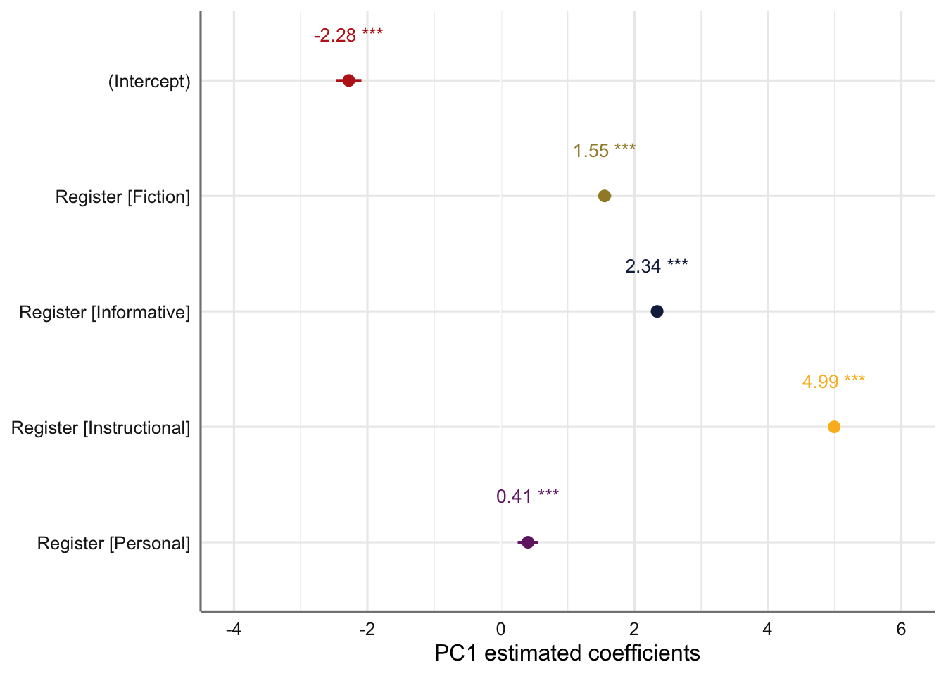
Code
#ggsave(here("plots", "TxB_PCA1_lmer_fixedeffects_Register.svg"), height = 3, width = 8)The emmeans and pairs functions are used to compare the estimated Dim1 scores for each register and to compare these to one another.
 Register       emmean    SE   df lower.CL upper.CL
 Conversation  -2.2793 0.102 11.6   -2.502   -2.056
 Fiction       -0.7267 0.106 13.9   -0.955   -0.498
 Informative    0.0603 0.104 12.7   -0.165    0.286
 Instructional  2.7141 0.101 11.3    2.492    2.937
 Personal      -1.8734 0.122 25.5   -2.125   -1.622

Degrees-of-freedom method: kenward-roger
Confidence level used: 0.95
Code
comparisons <- pairs(Register_results, adjust = "tukey")
comparisons
contrast estimate SE df t.ratio p.value
Conversation - Fiction -1.553 0.0508 1963 -30.535 <.0001
Conversation - Informative -2.340 0.0465 1961 -50.341 <.0001
Conversation - Instructional -4.993 0.0399 1961 -125.141 <.0001
Conversation - Personal -0.406 0.0791 1958 -5.134 <.0001
Fiction - Informative -0.787 0.0557 1962 -14.135 <.0001
Fiction - Instructional -3.441 0.0497 1962 -69.168 <.0001
Fiction - Personal 1.147 0.0840 1958 13.645 <.0001
Informative - Instructional -2.654 0.0447 1957 -59.399 <.0001
Informative - Personal 1.934 0.0816 1957 23.692 <.0001
Instructional - Personal 4.587 0.0780 1957 58.820 <.0001
Degrees-of-freedom method: kenward-roger
P value adjustment: tukey method for comparing a family of 5 estimates Code
#write_last_clip()
confint(comparisons)
contrast estimate SE df lower.CL upper.CL
Conversation - Fiction -1.553 0.0508 1963 -1.691 -1.414
Conversation - Informative -2.340 0.0465 1961 -2.466 -2.213
Conversation - Instructional -4.993 0.0399 1961 -5.102 -4.884
Conversation - Personal -0.406 0.0791 1958 -0.622 -0.190
Fiction - Informative -0.787 0.0557 1962 -0.939 -0.635
Fiction - Instructional -3.441 0.0497 1962 -3.577 -3.305
Fiction - Personal 1.147 0.0840 1958 0.917 1.376
Informative - Instructional -2.654 0.0447 1957 -2.776 -2.532
Informative - Personal 1.934 0.0816 1957 1.711 2.156
Instructional - Personal 4.587 0.0780 1957 4.374 4.800
Degrees-of-freedom method: kenward-roger
Confidence level used: 0.95
Conf-level adjustment: tukey method for comparing a family of 5 estimates Code
#write_last_clip()We can also visualise the estimated coefficients for the textbook series, which is modelled here as a random effect.
Code
plot_model(md1,
           type = "re", # Option to visualise random effects
           show.values=TRUE,
           show.p=TRUE,
           value.offset = .4,
           value.size = 3.5,
           colors = "bw",
           wrap.labels = 40,
           axis.title = "PC1 estimated coefficients") +
  theme_sjplot2()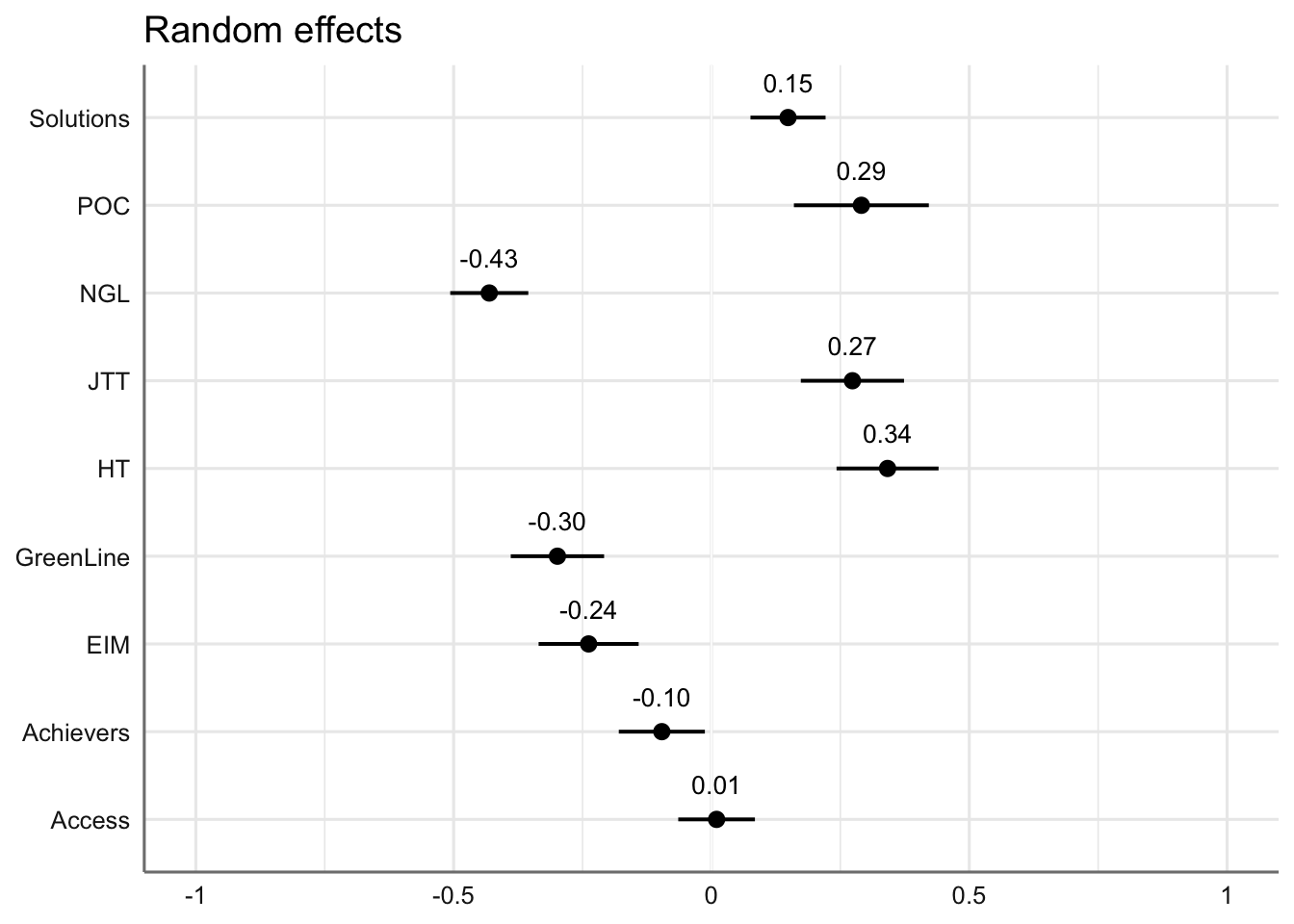
Code
#ggsave(here("plots", "TxB_PCA1_lmer_randomeffects.svg"), height = 3, width = 8)F.10.2 Dimension 2: ‘Involved vs. Informational Production’
Code
Data: res.ind
Models:
md2Register: PC2 ~ Register + (1 | Series)
md2Level: PC2 ~ Level + (1 | Series)
md2: PC2 ~ Register * Level + (1 | Series)
            npar    AIC    BIC  logLik deviance  Chisq Df Pr(>Chisq)
md2Register    7 6155.2 6194.3 -3070.6   6141.2
md2Level       7 7290.1 7329.2 -3638.1   7276.1    0.0  0
md2           27 5200.9 5351.6 -2573.4   5146.9 2129.2 20  < 2.2e-16 ***
---
Signif. codes:  0 '***' 0.001 '**' 0.01 '*' 0.05 '.' 0.1 ' ' 1
Code
tab_model(md2) # Marginal R2 = 0.723| PC 2 | |||
|---|---|---|---|
| Predictors | Estimates | CI | p |
| (Intercept) | 2.46 | 2.20 – 2.73 | <0.001 |
| Register [Fiction] | -1.80 | -2.14 – -1.46 | <0.001 |
| Register [Informative] | -3.44 | -3.79 – -3.08 | <0.001 |
| Register [Instructional] | -0.87 | -1.12 – -0.62 | <0.001 |
| Register [Personal] | -1.89 | -2.42 – -1.35 | <0.001 |
| Level [B] | -0.72 | -0.96 – -0.49 | <0.001 |
| Level [C] | -1.71 | -1.94 – -1.49 | <0.001 |
| Level [D] | -2.37 | -2.61 – -2.14 | <0.001 |
| Level [E] | -2.65 | -2.93 – -2.37 | <0.001 |
| Register [Fiction] × Level [B] |
-0.28 | -0.72 – 0.17 | 0.223 |
| Register [Informative] × Level [B] |
0.13 | -0.32 – 0.58 | 0.565 |
| Register [Instructional] × Level [B] |
0.44 | 0.11 – 0.77 | 0.009 |
| Register [Personal] × Level [B] |
0.53 | -0.14 – 1.20 | 0.120 |
| Register [Fiction] × Level [C] |
0.08 | -0.35 – 0.52 | 0.705 |
| Register [Informative] × Level [C] |
0.42 | -0.01 – 0.84 | 0.053 |
| Register [Instructional] × Level [C] |
1.11 | 0.80 – 1.43 | <0.001 |
| Register [Personal] × Level [C] |
0.59 | -0.07 – 1.26 | 0.081 |
| Register [Fiction] × Level [D] |
-0.01 | -0.44 – 0.42 | 0.972 |
| Register [Informative] × Level [D] |
0.49 | 0.07 – 0.91 | 0.024 |
| Register [Instructional] × Level [D] |
1.49 | 1.16 – 1.81 | <0.001 |
| Register [Personal] × Level [D] |
0.59 | -0.12 – 1.30 | 0.104 |
| Register [Fiction] × Level [E] |
0.42 | -0.04 – 0.87 | 0.072 |
| Register [Informative] × Level [E] |
0.39 | -0.07 – 0.86 | 0.099 |
| Register [Instructional] × Level [E] |
1.05 | 0.68 – 1.42 | <0.001 |
| Register [Personal] × Level [E] |
1.01 | 0.27 – 1.76 | 0.008 |
| Random Effects | |||
| σ2 | 0.80 | ||
| τ00Series | 0.09 | ||
| ICC | 0.10 | ||
| N Series | 9 | ||
| Observations | 1961 | ||
| Marginal R2 / Conditional R2 | 0.723 / 0.752 | ||
Code
# tab_model(md2Register) # Marginal R2 = 0.558
# tab_model(md2Level) # Marginal R2 = 0.228
Estimated coefficients of fixed effects on Dim2 scores:
Code
plot_model(md2,
           type = "est",
           show.intercept = TRUE,
           show.values=TRUE,
           show.p=TRUE,
           value.offset = .4,
           value.size = 3.5,
           colors = palette[c(1:3,8,7)],
           group.terms = c(1:5,1,1,1,1,2:5,2:5,2:5,2:5),
           title = "",
           wrap.labels = 40,
           axis.title = "PC2 estimated coefficients") +
theme_sjplot2() 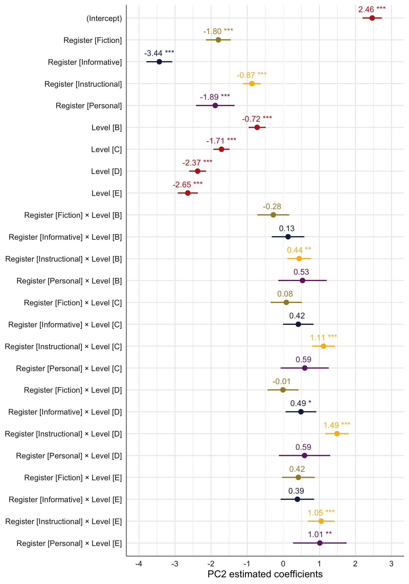
Code
#ggsave(here("plots", "TxB_PCA2_lmer_fixedeffects.svg"), height = 8, width = 8)Estimated coefficients of random effects on Dim2 scores:
Code
## Random intercepts
plot_model(md2,
           type = "re", # Option to visualise random effects
           show.values=TRUE,
           show.p=TRUE,
           value.offset = .4,
           value.size = 3.5,
           colors = "bw",
           wrap.labels = 40,
           axis.title = "PC2 estimated coefficients") +
  theme_sjplot2()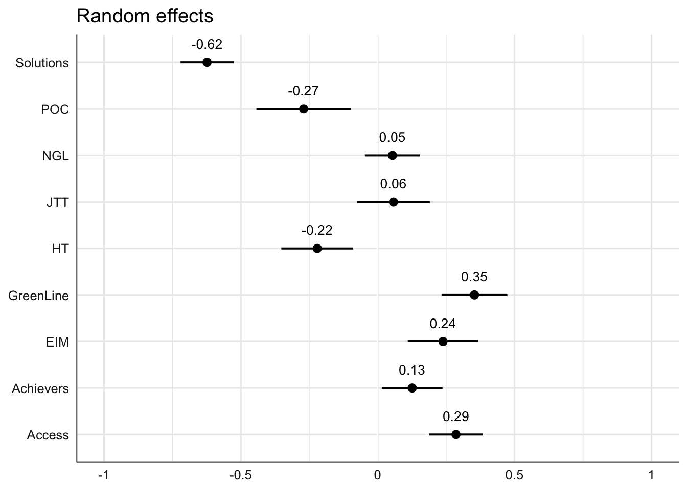
Code
#ggsave(here("plots", "TxB_PCA2_lmer_randomeffects.svg"), height = 3, width = 8)

# Textbook Country as a random effect variable
md2country <- lmer(PC2 ~ Register*Level + (1|Country), data = res.ind, REML = FALSE)

plot_model(md2country,
           type = "re", # Option to visualise random effects
           show.values=TRUE,
           show.p=TRUE,
           value.offset = .4,
           value.size = 3.5,
           colors = "bw",
           wrap.labels = 40,
           axis.title = "PC2 estimated coefficients") +
  theme_sjplot2()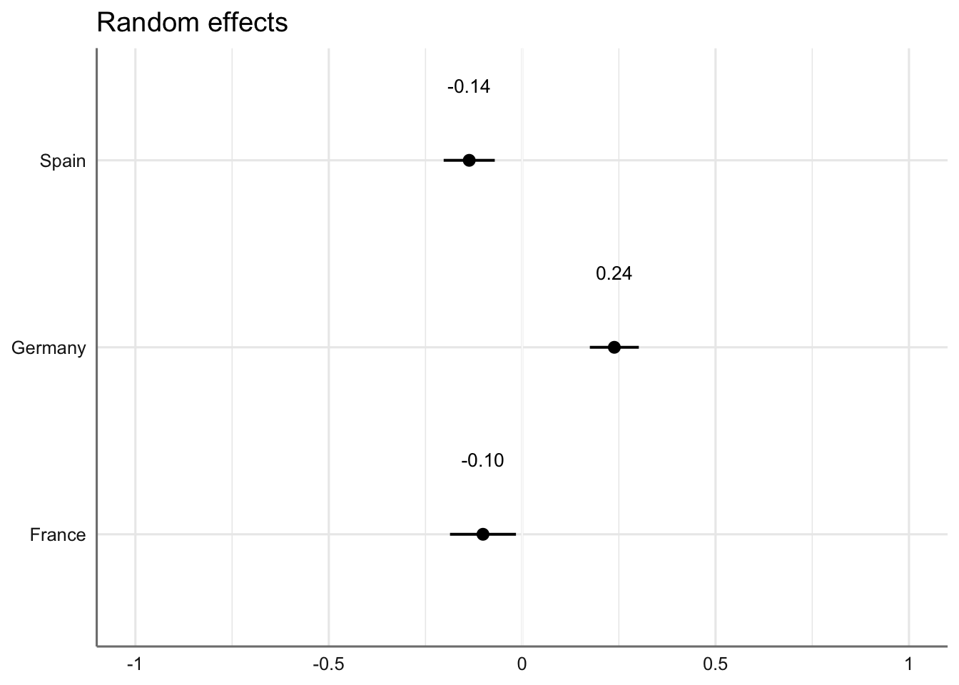
Code
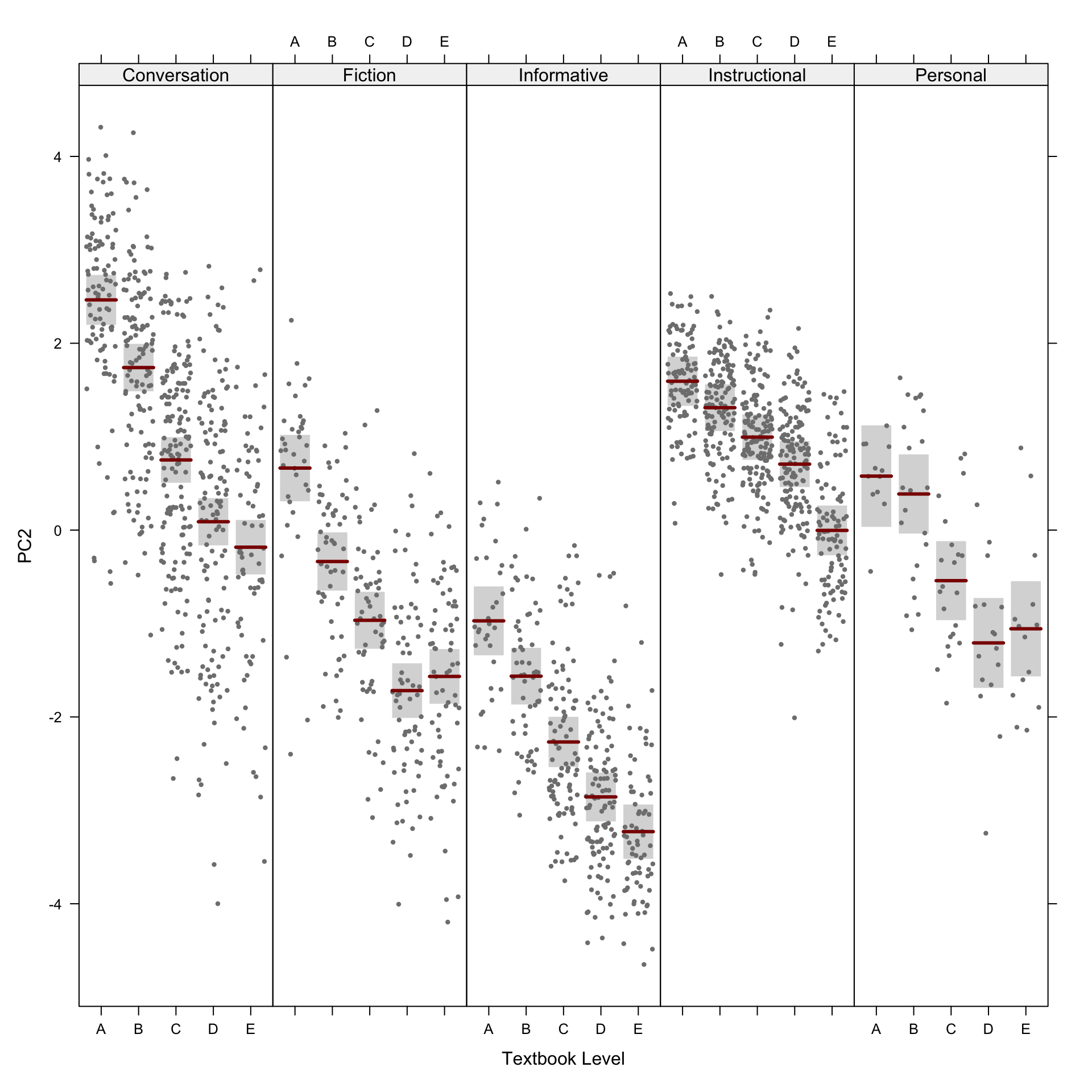
#ggsave(here("plots", "TxB_PCA2_lmer_randomeffects_country.svg"), height = 3, width = 8)The visreg function is used to visualise the distributions of the modelled Dim2 scores.
Code
Code
#dev.off()We also examine potential interactions between textbook series, proficiency level, and Dim2 scores.
Code

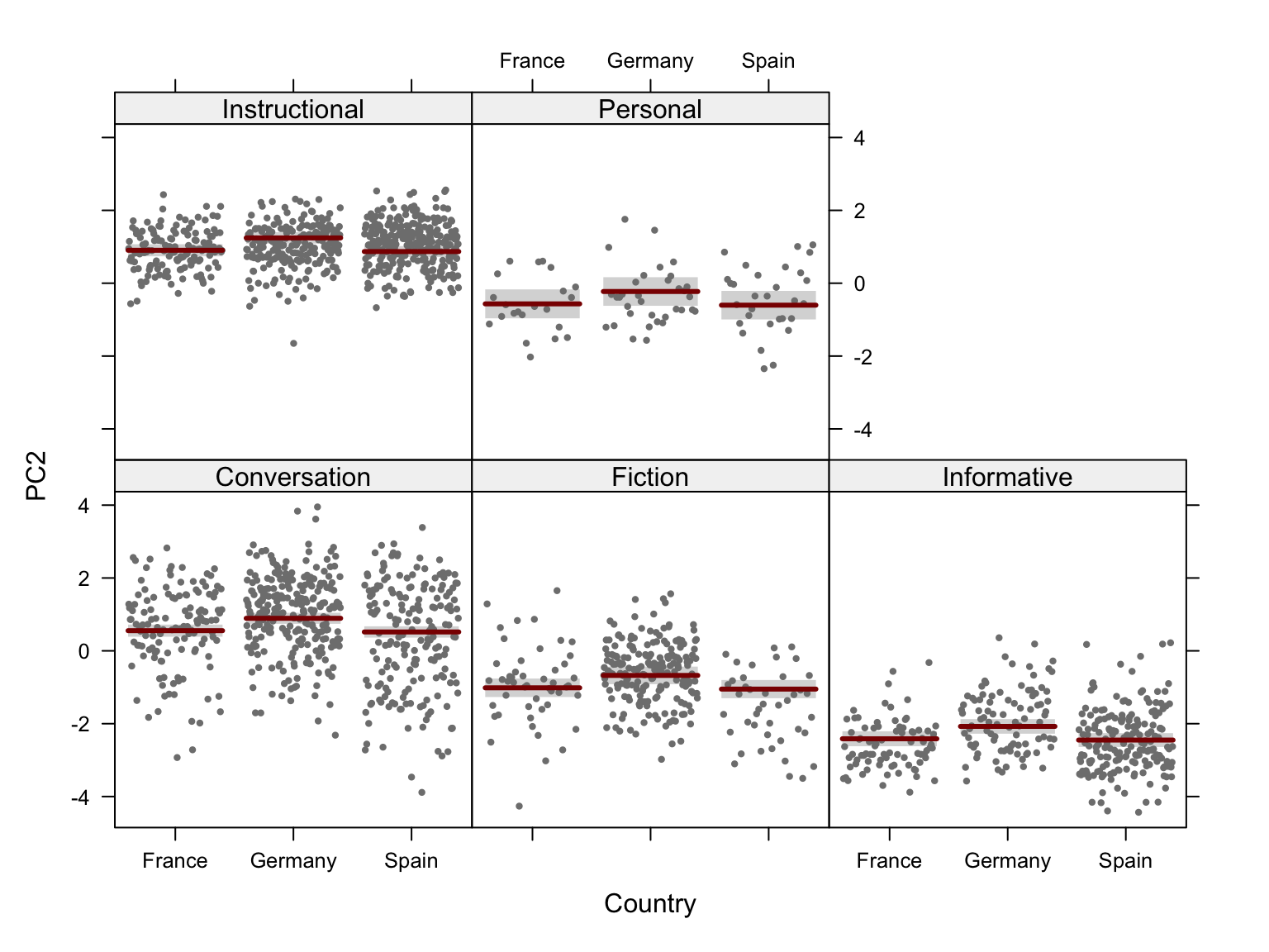
Finally, we examine potential interactions between country of use of the textbook, register, and Dim2 scores.
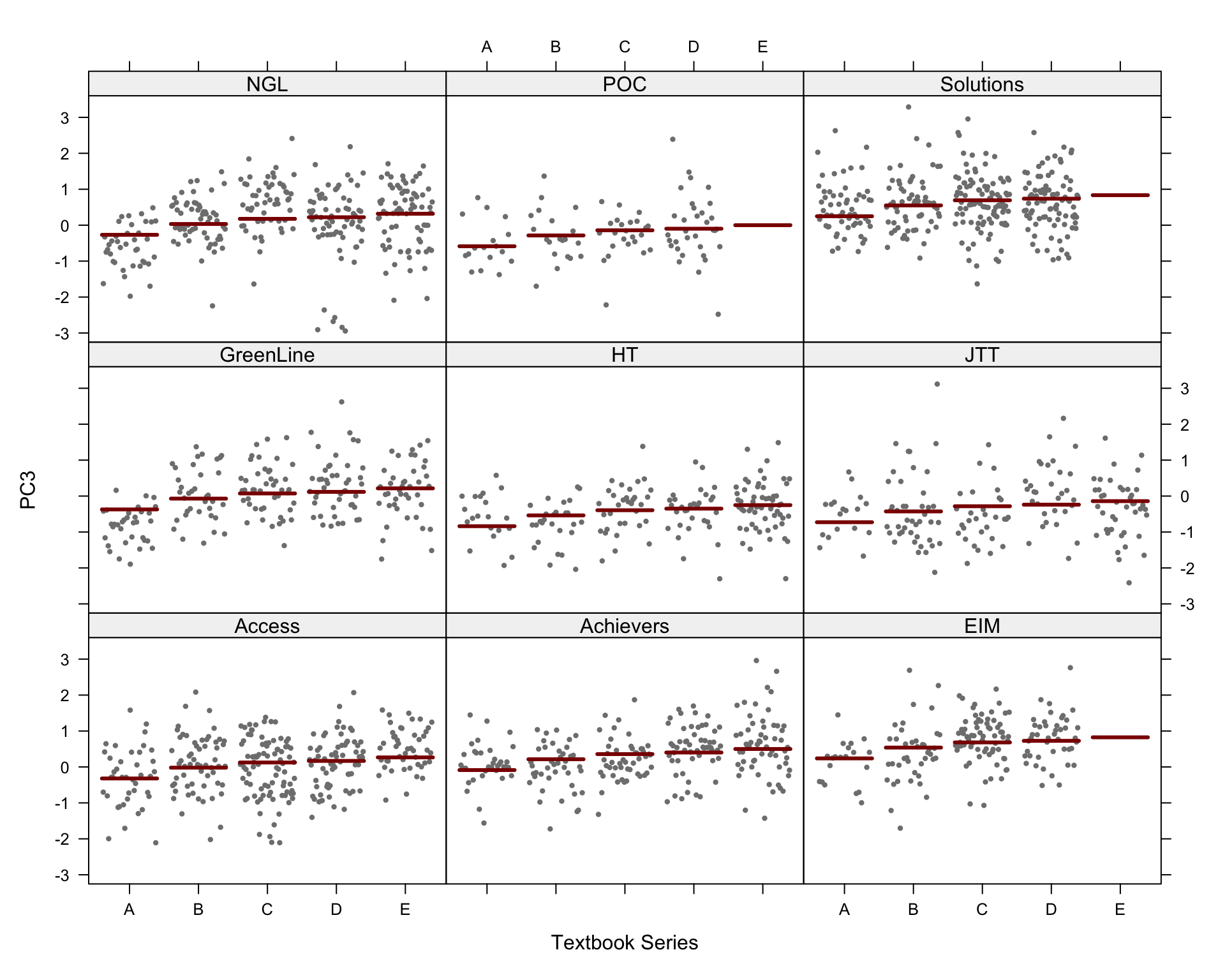
F.10.3 Dimension 3: ‘Narrative vs. factual discourse’
Code
Data: res.ind
Models:
md3Register: PC3 ~ Register + (1 | Series)
md3Level: PC3 ~ Level + (1 | Series)
md3: PC3 ~ Register * Level + (1 | Series)
            npar    AIC    BIC  logLik deviance  Chisq Df Pr(>Chisq)
md3Register    7 5139.9 5179.0 -2563.0   5125.9
md3Level       7 5528.8 5567.9 -2757.4   5514.8   0.00  0
md3           27 4582.6 4733.3 -2264.3   4528.6 986.21 20  < 2.2e-16 ***
---
Signif. codes:  0 '***' 0.001 '**' 0.01 '*' 0.05 '.' 0.1 ' ' 1
Code
tab_model(md3) # Marginal R2 = 0.436| PC 3 | |||
|---|---|---|---|
| Predictors | Estimates | CI | p |
| (Intercept) | -1.33 | -1.62 – -1.04 | <0.001 |
| Register [Fiction] | 0.79 | 0.50 – 1.08 | <0.001 |
| Register [Informative] | -0.79 | -1.10 – -0.49 | <0.001 |
| Register [Instructional] | 1.03 | 0.82 – 1.24 | <0.001 |
| Register [Personal] | 0.19 | -0.27 – 0.65 | 0.411 |
| Level [B] | 0.97 | 0.77 – 1.17 | <0.001 |
| Level [C] | 1.39 | 1.20 – 1.58 | <0.001 |
| Level [D] | 1.50 | 1.30 – 1.70 | <0.001 |
| Level [E] | 1.60 | 1.36 – 1.83 | <0.001 |
| Register [Fiction] × Level [B] |
0.55 | 0.17 – 0.93 | 0.004 |
| Register [Informative] × Level [B] |
-0.13 | -0.52 – 0.25 | 0.504 |
| Register [Instructional] × Level [B] |
-0.67 | -0.95 – -0.39 | <0.001 |
| Register [Personal] × Level [B] |
-0.34 | -0.91 – 0.23 | 0.242 |
| Register [Fiction] × Level [C] |
0.78 | 0.41 – 1.15 | <0.001 |
| Register [Informative] × Level [C] |
-0.17 | -0.53 – 0.19 | 0.362 |
| Register [Instructional] × Level [C] |
-0.94 | -1.21 – -0.68 | <0.001 |
| Register [Personal] × Level [C] |
0.17 | -0.40 – 0.74 | 0.568 |
| Register [Fiction] × Level [D] |
0.34 | -0.03 – 0.70 | 0.073 |
| Register [Informative] × Level [D] |
0.01 | -0.35 – 0.37 | 0.953 |
| Register [Instructional] × Level [D] |
-1.01 | -1.29 – -0.73 | <0.001 |
| Register [Personal] × Level [D] |
0.02 | -0.58 – 0.63 | 0.939 |
| Register [Fiction] × Level [E] |
0.23 | -0.15 – 0.62 | 0.238 |
| Register [Informative] × Level [E] |
-0.18 | -0.58 – 0.21 | 0.364 |
| Register [Instructional] × Level [E] |
-1.01 | -1.32 – -0.70 | <0.001 |
| Register [Personal] × Level [E] |
-0.21 | -0.84 – 0.43 | 0.520 |
| Random Effects | |||
| σ2 | 0.58 | ||
| τ00Series | 0.14 | ||
| ICC | 0.19 | ||
| N Series | 9 | ||
| Observations | 1961 | ||
| Marginal R2 / Conditional R2 | 0.436 / 0.543 | ||
Code
# tab_model(md3Register) # Marginal R2 = 0.272
# tab_model(md3Level) # Marginal R2 = 0.119

# Plot of fixed effects:
plot_model(md3,
           type = "est",
           show.intercept = TRUE,
           show.values=TRUE,
           show.p=TRUE,
           value.offset = .4,
           value.size = 3.5,
           colors = palette[c(1:3,8,7)],
           group.terms = c(1:5,1,1,1,1,2:5,2:5,2:5,2:5),
           title = "",
           wrap.labels = 40,
           axis.title = "PC3 estimated coefficients") +
theme_sjplot2() 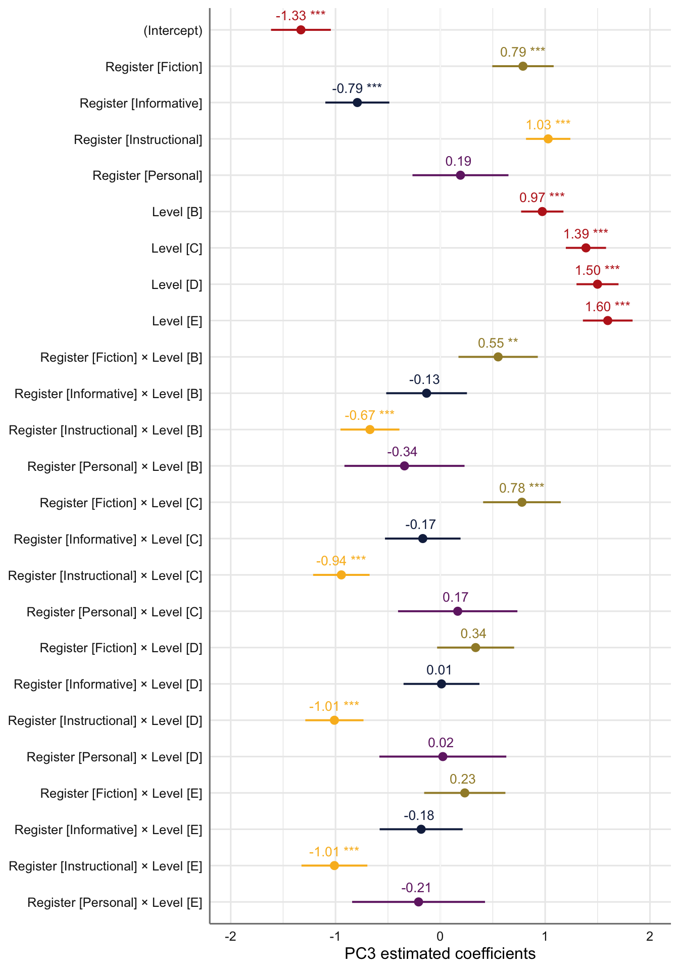
Code
#ggsave(here("plots", "TxB_PCA3_lmer_fixedeffects.svg"), height = 8, width = 8)# Plot of random effects:
plot_model(md3,
type = "re", # Option to visualise random effects
show.values=TRUE,
show.p=TRUE,
value.offset = .4,
value.size = 3.5,
color = "bw",
wrap.labels = 40,
axis.title = "PC3 estimated coefficients") +
theme_sjplot2()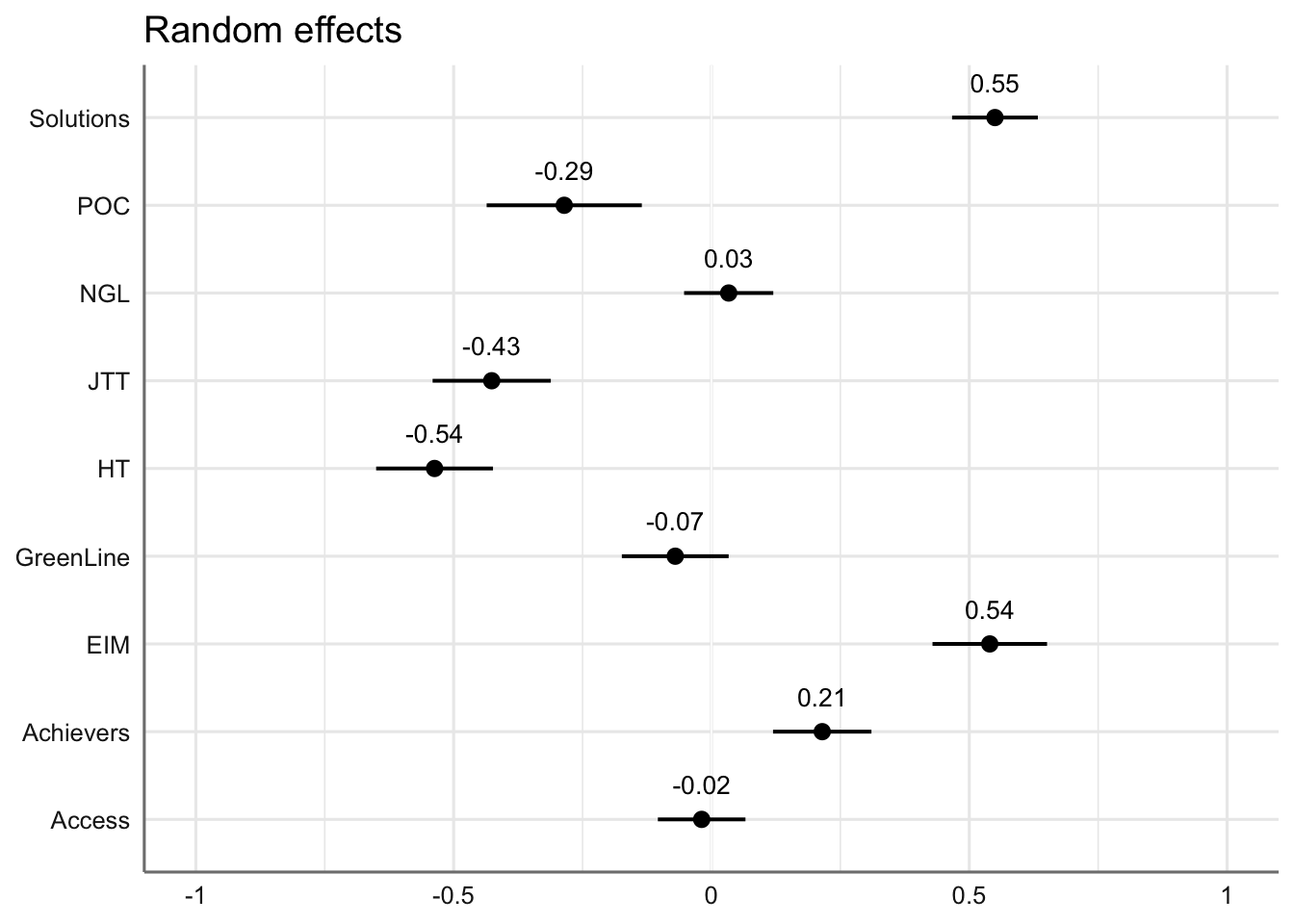
#ggsave(here("plots", "TxB_PCA3_lmer_randomeffects.svg"), height = 3, width = 8)Code
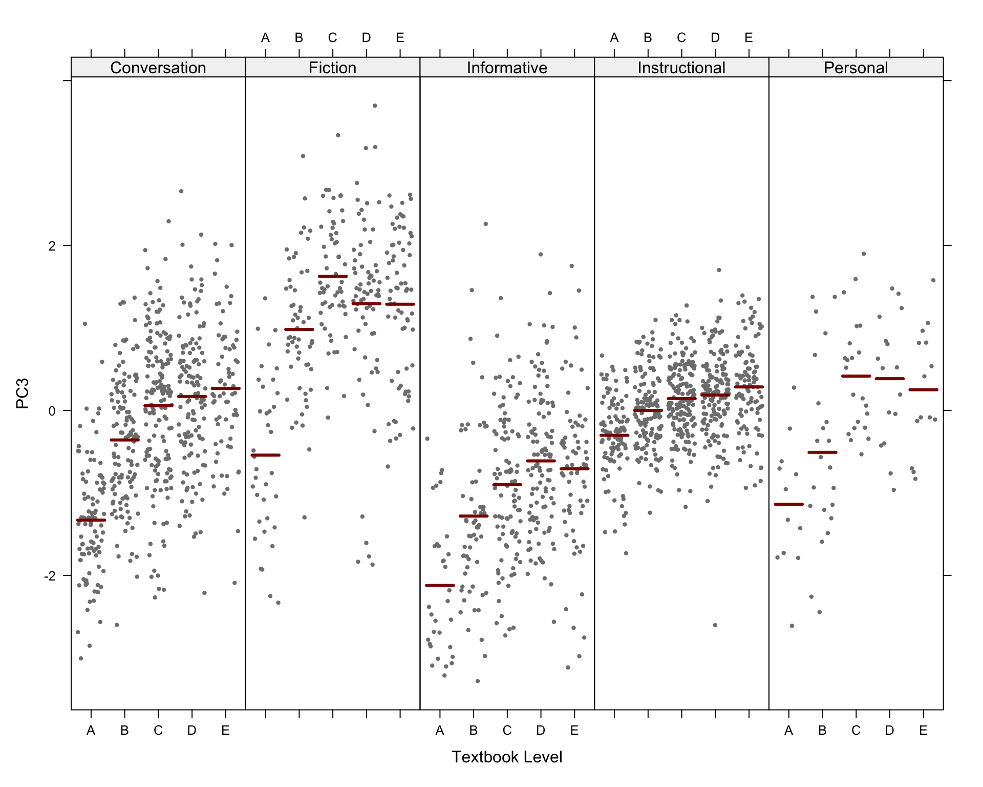
Code
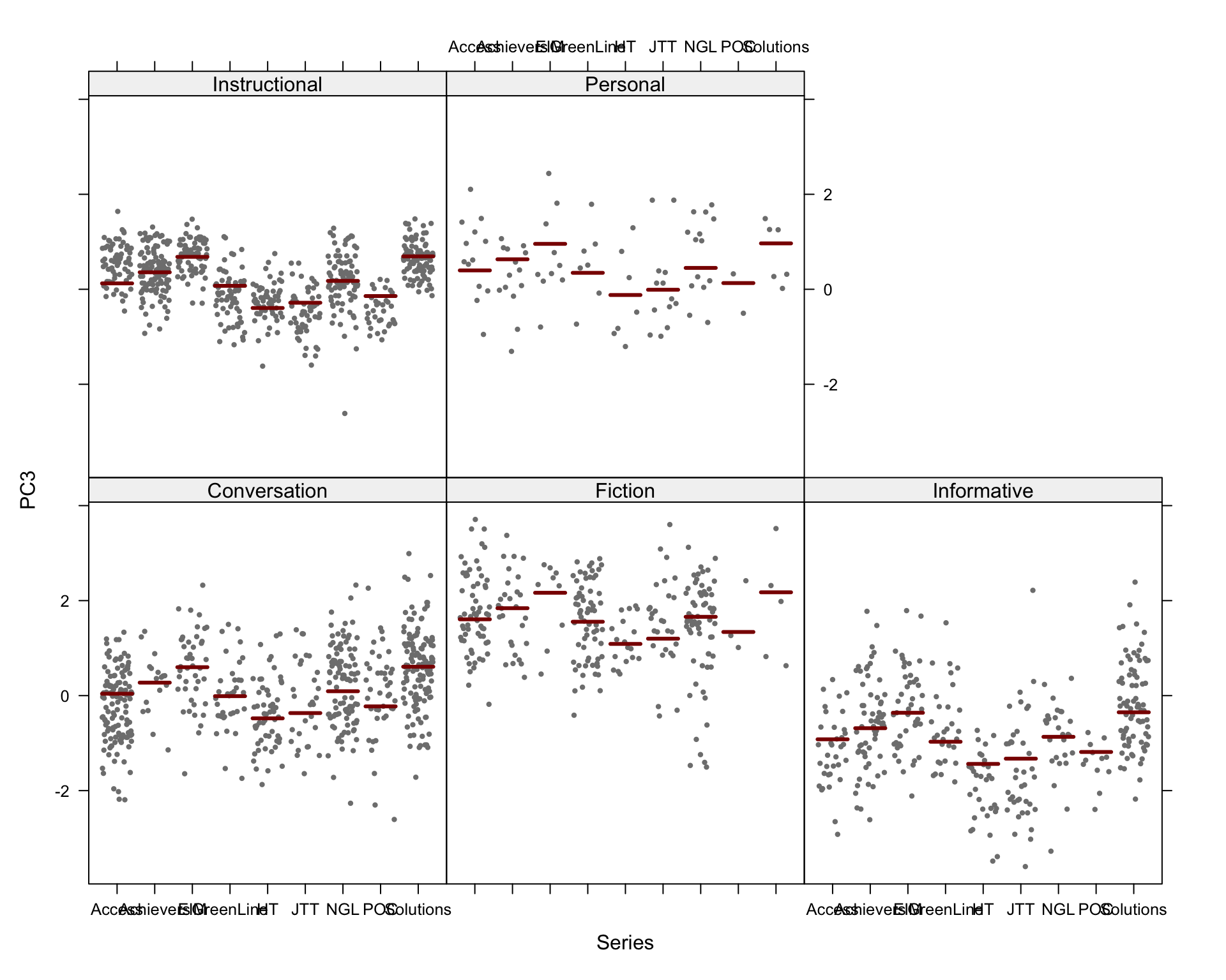
Code
F.10.4 Dimension 4: ‘Informational compression vs. elaboration’
Code
Data: res.ind
Models:
md4Register: PC4 ~ Register + (1 | Series)
md4Level: PC4 ~ Level + (1 | Series)
md4: PC4 ~ Register * Level + (1 | Series)
            npar    AIC    BIC  logLik deviance  Chisq Df Pr(>Chisq)
md4Register    7 5034.0 5073.0 -2510.0   5020.0
md4Level       7 5043.6 5082.7 -2514.8   5029.6   0.00  0
md4           27 4372.1 4522.8 -2159.1   4318.1 711.52 20  < 2.2e-16 ***
---
Signif. codes:  0 '***' 0.001 '**' 0.01 '*' 0.05 '.' 0.1 ' ' 1
Code
tab_model(md4) # Marginal R2 = 0.426| PC 4 | |||
|---|---|---|---|
| Predictors | Estimates | CI | p |
| (Intercept) | 0.76 | 0.56 – 0.96 | <0.001 |
| Register [Fiction] | 0.72 | 0.44 – 1.00 | <0.001 |
| Register [Informative] | 0.20 | -0.09 – 0.49 | 0.176 |
| Register [Instructional] | -0.23 | -0.43 – -0.03 | 0.023 |
| Register [Personal] | 0.49 | 0.06 – 0.93 | 0.026 |
| Level [B] | -0.67 | -0.87 – -0.48 | <0.001 |
| Level [C] | -1.14 | -1.32 – -0.96 | <0.001 |
| Level [D] | -1.42 | -1.61 – -1.23 | <0.001 |
| Level [E] | -1.76 | -1.99 – -1.54 | <0.001 |
| Register [Fiction] × Level [B] |
0.97 | 0.61 – 1.33 | <0.001 |
| Register [Informative] × Level [B] |
0.22 | -0.14 – 0.59 | 0.230 |
| Register [Instructional] × Level [B] |
0.21 | -0.06 – 0.47 | 0.130 |
| Register [Personal] × Level [B] |
-0.02 | -0.57 – 0.52 | 0.930 |
| Register [Fiction] × Level [C] |
0.85 | 0.50 – 1.20 | <0.001 |
| Register [Informative] × Level [C] |
0.25 | -0.09 – 0.59 | 0.156 |
| Register [Instructional] × Level [C] |
0.37 | 0.11 – 0.62 | 0.005 |
| Register [Personal] × Level [C] |
-0.26 | -0.80 – 0.28 | 0.343 |
| Register [Fiction] × Level [D] |
0.65 | 0.30 – 1.00 | <0.001 |
| Register [Informative] × Level [D] |
0.34 | -0.00 – 0.68 | 0.053 |
| Register [Instructional] × Level [D] |
0.47 | 0.20 – 0.73 | 0.001 |
| Register [Personal] × Level [D] |
-0.43 | -1.01 – 0.14 | 0.140 |
| Register [Fiction] × Level [E] |
0.82 | 0.45 – 1.19 | <0.001 |
| Register [Informative] × Level [E] |
0.42 | 0.05 – 0.80 | 0.027 |
| Register [Instructional] × Level [E] |
0.44 | 0.14 – 0.74 | 0.004 |
| Register [Personal] × Level [E] |
-0.55 | -1.15 – 0.05 | 0.072 |
| Random Effects | |||
| σ2 | 0.52 | ||
| τ00Series | 0.05 | ||
| ICC | 0.08 | ||
| N Series | 9 | ||
| Observations | 1961 | ||
| Marginal R2 / Conditional R2 | 0.426 / 0.472 | ||
Code
# tab_model(md4Register) # Marginal R2 = 0.203
# tab_model(md4Level) # Marginal R2 = 0.187

# Plot of fixed effects:
plot_model(md4,
           type = "est",
           show.intercept = TRUE,
           show.values=TRUE,
           show.p=TRUE,
           value.offset = .4,
           value.size = 3.5,
           colors = palette[c(1:3,8,7)],
           group.terms = c(1:5,1,1,1,1,2:5,2:5,2:5,2:5),
           title = "",
           wrap.labels = 40,
           axis.title = "PC4 estimated coefficients") +
theme_sjplot2() 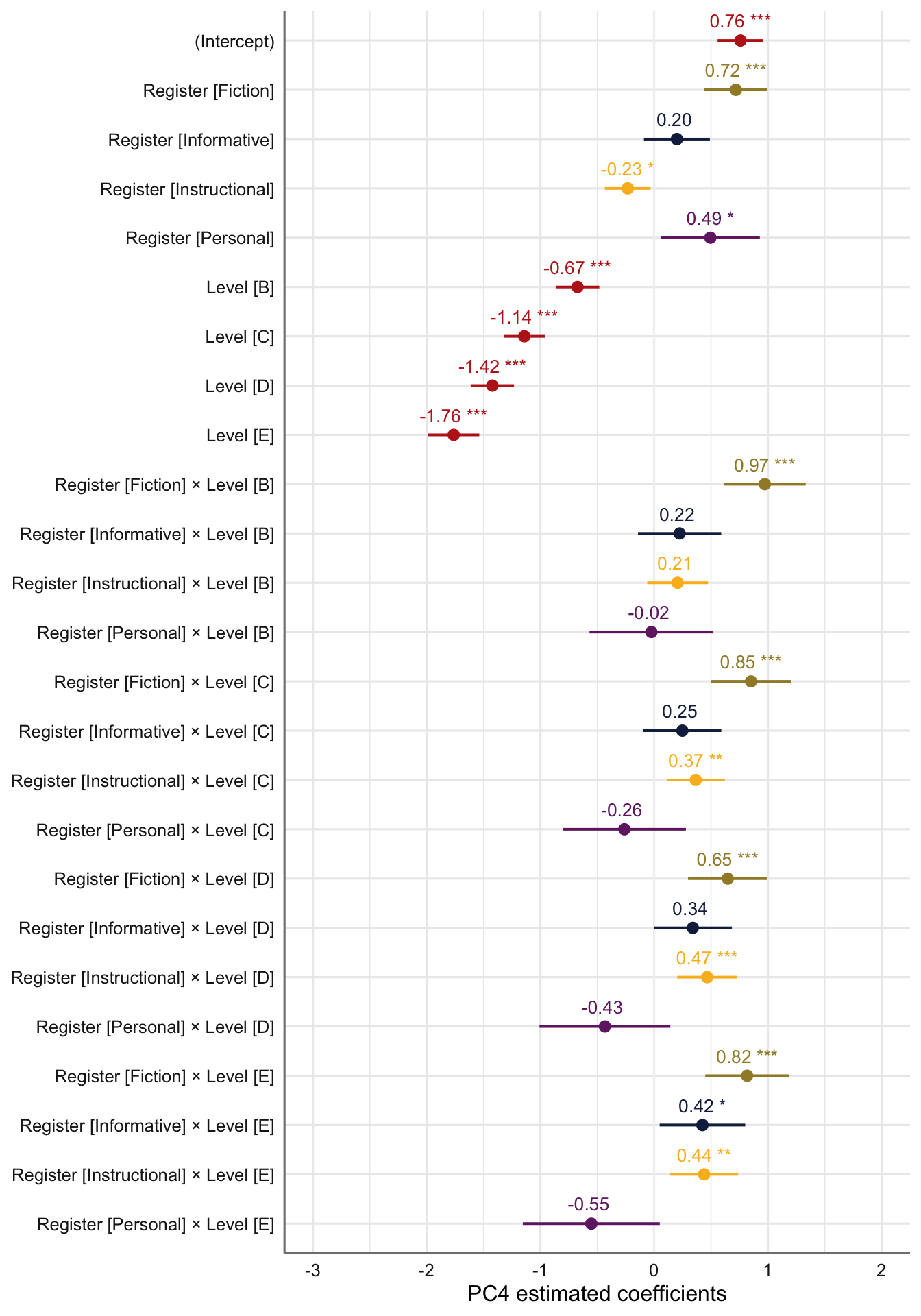
Code
#ggsave(here("plots", "TxB_PCA4_lmer_fixedeffects.svg"), height = 8, width = 8)Code
# Plot of random effects:
plot_model(md4,
           type = "re", # Option to visualise random effects
           show.values=TRUE,
           show.p=TRUE,
           value.offset = .4,
           value.size = 3.5,
           color = "bw",
           wrap.labels = 40,
           axis.title = "PC4 estimated coefficients") +
  theme_sjplot2()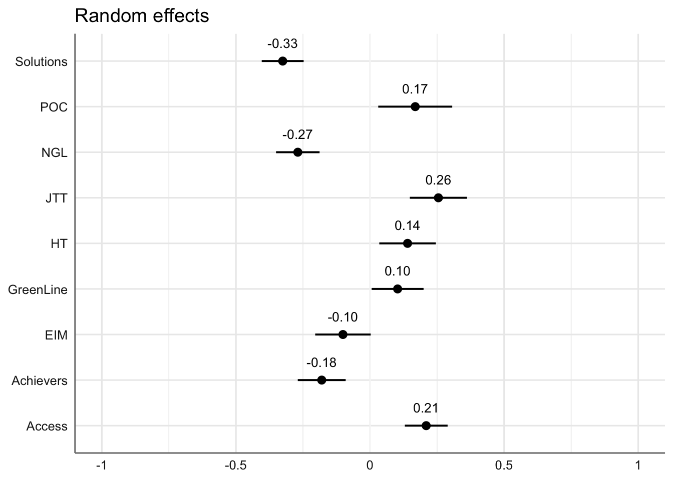
Code
#ggsave(here("plots", "TxB_PCA4_lmer_randomeffects.svg"), height = 3, width = 8)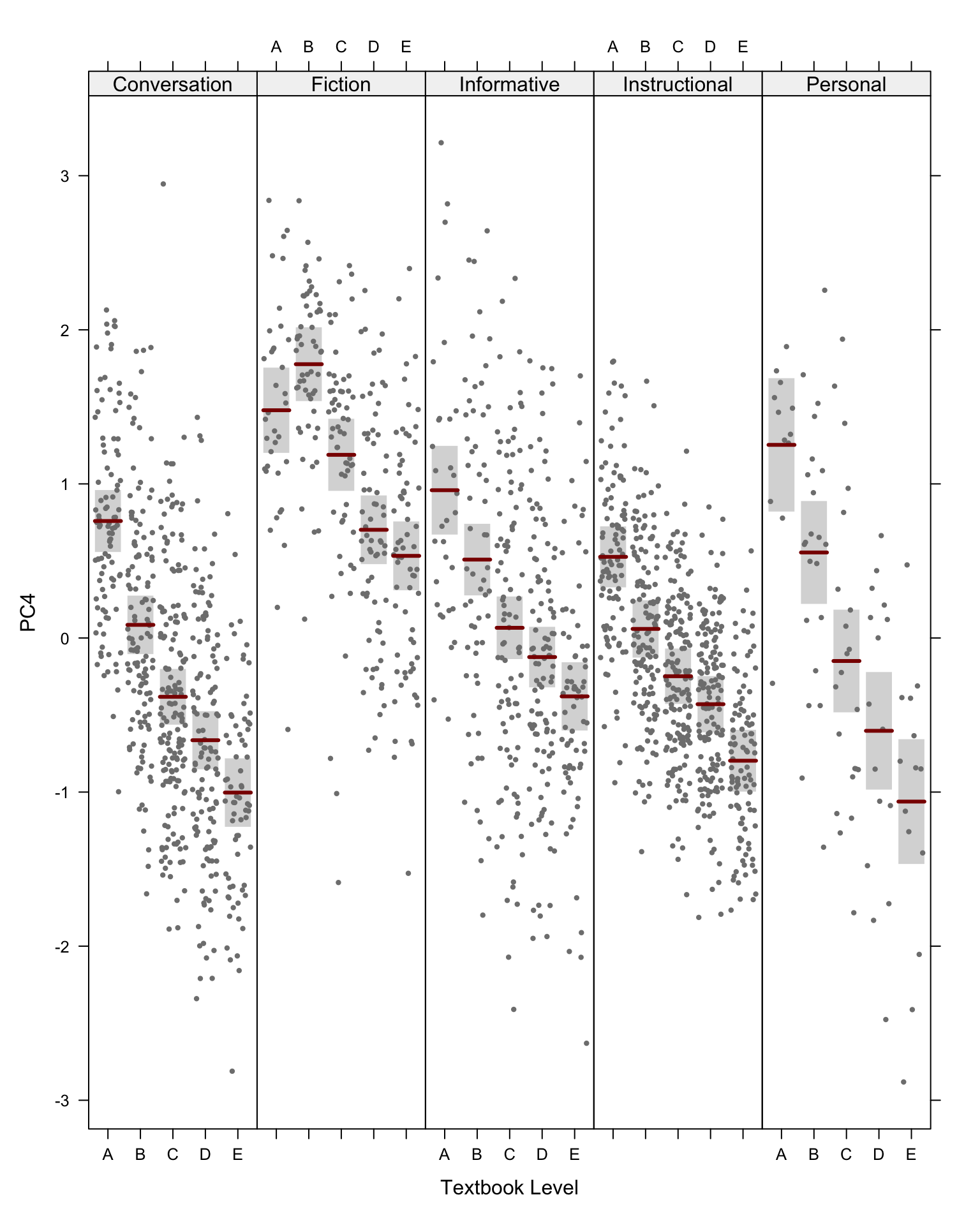
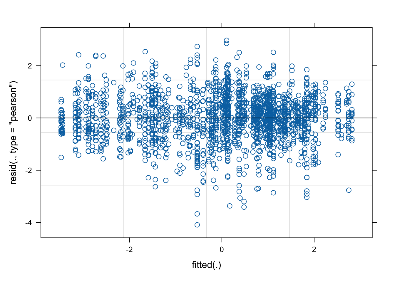
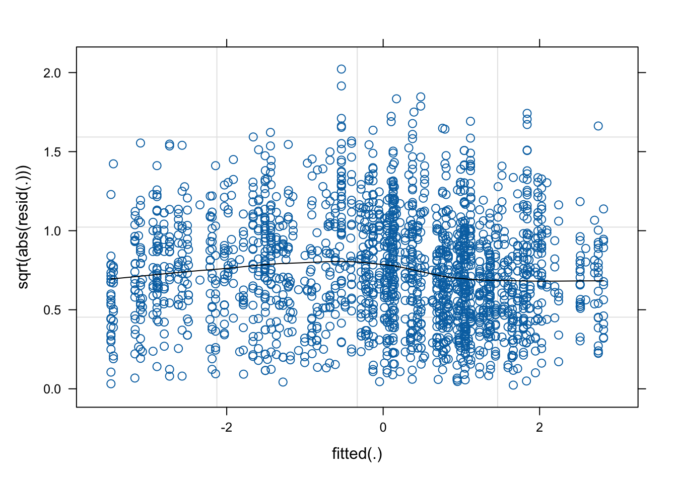
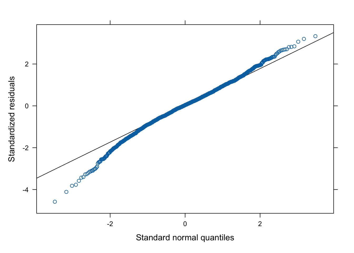
F.10.5 Testing model assumptions
This chunk can be used to check the assumptions of all of the models computed above. In the following example, we examine the final model selected to predict Dim2 scores.
F.11 Packages used in this script
F.11.1 Package names and versions
R version 4.4.1 (2024-06-14)
Platform: aarch64-apple-darwin20
Running under: macOS Sonoma 14.5

Matrix products: default
BLAS:   /Library/Frameworks/R.framework/Versions/4.4-arm64/Resources/lib/libRblas.0.dylib
LAPACK: /Library/Frameworks/R.framework/Versions/4.4-arm64/Resources/lib/libRlapack.dylib;  LAPACK version 3.12.0

locale:
[1] en_US.UTF-8/en_US.UTF-8/en_US.UTF-8/C/en_US.UTF-8/en_US.UTF-8

time zone: Europe/Madrid
tzcode source: internal

attached base packages:
[1] stats     graphics  grDevices datasets  utils     methods   base

other attached packages:
 [1] visreg_2.7.0      lubridate_1.9.3   stringr_1.5.1     dplyr_1.1.4
 [5] purrr_1.0.2       readr_2.1.5       tidyr_1.3.1       tibble_3.2.1
 [9] tidyverse_2.0.0   sjPlot_2.8.16     psych_2.4.6.26    PCAtools_2.14.0
[13] ggrepel_0.9.5     patchwork_1.2.0   lme4_1.1-35.5     Matrix_1.7-0
[17] knitr_1.48        here_1.0.1        ggthemes_5.1.0    forcats_1.0.0
[21] factoextra_1.0.7  emmeans_1.10.3    DescTools_0.99.54 cowplot_1.1.3
[25] caret_6.0-94      lattice_0.22-6    ggplot2_3.5.1

loaded via a namespace (and not attached):
  [1] rstudioapi_0.16.0         jsonlite_1.8.8
  [3] datawizard_0.12.1         magrittr_2.0.3
  [5] estimability_1.5.1        nloptr_2.1.1
  [7] rmarkdown_2.27            zlibbioc_1.50.0
  [9] vctrs_0.6.5               minqa_1.2.7
 [11] DelayedMatrixStats_1.26.0 htmltools_0.5.8.1
 [13] S4Arrays_1.4.1            cellranger_1.1.0
 [15] sjmisc_2.8.10             SparseArray_1.4.8
 [17] pROC_1.18.5               parallelly_1.37.1
 [19] htmlwidgets_1.6.4         plyr_1.8.9
 [21] rootSolve_1.8.2.4         lifecycle_1.0.4
 [23] iterators_1.0.14          pkgconfig_2.0.3
 [25] sjlabelled_1.2.0          rsvd_1.0.5
 [27] R6_2.5.1                  fastmap_1.2.0
 [29] MatrixGenerics_1.16.0     future_1.33.2
 [31] digest_0.6.36             Exact_3.2
 [33] colorspace_2.1-0          S4Vectors_0.42.1
 [35] rprojroot_2.0.4           dqrng_0.4.1
 [37] irlba_2.3.5.1             beachmat_2.20.0
 [39] fansi_1.0.6               timechange_0.3.0
 [41] httr_1.4.7                abind_1.4-5
 [43] compiler_4.4.1            proxy_0.4-27
 [45] withr_3.0.0               BiocParallel_1.38.0
 [47] performance_0.12.2        MASS_7.3-60.2
 [49] lava_1.8.0                sjstats_0.19.0
 [51] DelayedArray_0.30.1       gld_2.6.6
 [53] ModelMetrics_1.2.2.2      tools_4.4.1
 [55] future.apply_1.11.2       nnet_7.3-19
 [57] glue_1.7.0                nlme_3.1-164
 [59] grid_4.4.1                reshape2_1.4.4
 [61] generics_0.1.3            recipes_1.1.0
 [63] gtable_0.3.5              tzdb_0.4.0
 [65] class_7.3-22              hms_1.1.3
 [67] data.table_1.15.4         lmom_3.0
 [69] BiocSingular_1.20.0       ScaledMatrix_1.12.0
 [71] utf8_1.2.4                XVector_0.44.0
 [73] BiocGenerics_0.50.0       foreach_1.5.2
 [75] pillar_1.9.0              splines_4.4.1
 [77] renv_1.0.3                survival_3.6-4
 [79] tidyselect_1.2.1          IRanges_2.38.1
 [81] stats4_4.4.1              xfun_0.46
 [83] expm_0.999-9              hardhat_1.4.0
 [85] timeDate_4032.109         matrixStats_1.3.0
 [87] stringi_1.8.4             yaml_2.3.9
 [89] boot_1.3-30               evaluate_0.24.0
 [91] codetools_0.2-20          BiocManager_1.30.23
 [93] cli_3.6.3                 rpart_4.1.23
 [95] xtable_1.8-4              munsell_0.5.1
 [97] Rcpp_1.0.13               readxl_1.4.3
 [99] globals_0.16.3            ggeffects_1.7.0
[101] coda_0.19-4.1             parallel_4.4.1
[103] gower_1.0.1               sparseMatrixStats_1.16.0
[105] listenv_0.9.1             mvtnorm_1.2-5
[107] ipred_0.9-15              scales_1.3.0
[109] prodlim_2024.06.25        e1071_1.7-14
[111] insight_0.20.2            crayon_1.5.3
[113] rlang_1.1.4               mnormt_2.1.1
F.11.2 Package references
[1] J. B. Arnold. ggthemes: Extra Themes, Scales and Geoms for ggplot2. R package version 5.1.0. 2024. https://jrnold.github.io/ggthemes/.
[2] D. Bates, M. Mächler, B. Bolker, et al. “Fitting Linear Mixed-Effects Models Using lme4”. In: Journal of Statistical Software 67.1 (2015), pp. 1-48. DOI: 10.18637/jss.v067.i01.
[3] D. Bates, M. Maechler, B. Bolker, et al. lme4: Linear Mixed-Effects Models using Eigen and S4. R package version 1.1-35.5. 2024. https://github.com/lme4/lme4/.
[4] D. Bates, M. Maechler, and M. Jagan. Matrix: Sparse and Dense Matrix Classes and Methods. R package version 1.7-0. 2024. https://Matrix.R-forge.R-project.org.
[5] K. Blighe and A. Lun. PCAtools: Everything Principal Components Analysis. R package version 2.14.0. 2023. DOI: 10.18129/B9.bioc.PCAtools. https://bioconductor.org/packages/PCAtools.
[6] P. Breheny and W. Burchett. visreg: Visualization of Regression Models. R package version 2.7.0. 2020. http://pbreheny.github.io/visreg.
[7] P. Breheny and W. Burchett. “Visualization of Regression Models Using visreg”. In: The R Journal 9.2 (2017), pp. 56-71.
[8] G. Grolemund and H. Wickham. “Dates and Times Made Easy with lubridate”. In: Journal of Statistical Software 40.3 (2011), pp. 1-25. https://www.jstatsoft.org/v40/i03/.
[9] A. Kassambara and F. Mundt. factoextra: Extract and Visualize the Results of Multivariate Data Analyses. R package version 1.0.7. 2020. http://www.sthda.com/english/rpkgs/factoextra.
[10] M. Kuhn. caret: Classification and Regression Training. R package version 6.0-94. 2023. https://github.com/topepo/caret/.
[11] Kuhn and Max. “Building Predictive Models in R Using the caret Package”. In: Journal of Statistical Software 28.5 (2008), p. 1–26. DOI: 10.18637/jss.v028.i05. https://www.jstatsoft.org/index.php/jss/article/view/v028i05.
[12] R. V. Lenth. emmeans: Estimated Marginal Means, aka Least-Squares Means. R package version 1.10.3. 2024. https://rvlenth.github.io/emmeans/.
[13] D. Lüdecke. sjPlot: Data Visualization for Statistics in Social Science. R package version 2.8.16. 2024. https://strengejacke.github.io/sjPlot/.
[14] K. Müller. here: A Simpler Way to Find Your Files. R package version 1.0.1. 2020. https://here.r-lib.org/.
[15] K. Müller and H. Wickham. tibble: Simple Data Frames. R package version 3.2.1. 2023. https://tibble.tidyverse.org/.
[16] T. L. Pedersen. patchwork: The Composer of Plots. R package version 1.2.0. 2024. https://patchwork.data-imaginist.com.
[17] R Core Team. R: A Language and Environment for Statistical Computing. R Foundation for Statistical Computing. Vienna, Austria, 2024. https://www.R-project.org/.
[18] W. Revelle. psych: Procedures for Psychological, Psychometric, and Personality Research. R package version 2.4.6.26. 2024. https://personality-project.org/r/psych/.
[19] D. Sarkar. Lattice: Multivariate Data Visualization with R. New York: Springer, 2008. ISBN: 978-0-387-75968-5. http://lmdvr.r-forge.r-project.org.
[20] D. Sarkar. lattice: Trellis Graphics for R. R package version 0.22-6. 2024. https://lattice.r-forge.r-project.org/.
[21] A. Signorell. DescTools: Tools for Descriptive Statistics. R package version 0.99.54. 2024. https://andrisignorell.github.io/DescTools/.
[22] K. Slowikowski. ggrepel: Automatically Position Non-Overlapping Text Labels with ggplot2. R package version 0.9.5. 2024. https://ggrepel.slowkow.com/.
[23] V. Spinu, G. Grolemund, and H. Wickham. lubridate: Make Dealing with Dates a Little Easier. R package version 1.9.3. 2023. https://lubridate.tidyverse.org.
[24] H. Wickham. forcats: Tools for Working with Categorical Variables (Factors). R package version 1.0.0. 2023. https://forcats.tidyverse.org/.
[25] H. Wickham. ggplot2: Elegant Graphics for Data Analysis. Springer-Verlag New York, 2016. ISBN: 978-3-319-24277-4. https://ggplot2.tidyverse.org.
[26] H. Wickham. stringr: Simple, Consistent Wrappers for Common String Operations. R package version 1.5.1. 2023. https://stringr.tidyverse.org.
[27] H. Wickham. tidyverse: Easily Install and Load the Tidyverse. R package version 2.0.0. 2023. https://tidyverse.tidyverse.org.
[28] H. Wickham, M. Averick, J. Bryan, et al. “Welcome to the tidyverse”. In: Journal of Open Source Software 4.43 (2019), p. 1686. DOI: 10.21105/joss.01686.
[29] H. Wickham, W. Chang, L. Henry, et al. ggplot2: Create Elegant Data Visualisations Using the Grammar of Graphics. R package version 3.5.1. 2024. https://ggplot2.tidyverse.org.
[30] H. Wickham, R. François, L. Henry, et al. dplyr: A Grammar of Data Manipulation. R package version 1.1.4. 2023. https://dplyr.tidyverse.org.
[31] H. Wickham and L. Henry. purrr: Functional Programming Tools. R package version 1.0.2. 2023. https://purrr.tidyverse.org/.
[32] H. Wickham, J. Hester, and J. Bryan. readr: Read Rectangular Text Data. R package version 2.1.5. 2024. https://readr.tidyverse.org.
[33] H. Wickham, D. Vaughan, and M. Girlich. tidyr: Tidy Messy Data. R package version 1.3.1. 2024. https://tidyr.tidyverse.org.
[34] C. O. Wilke. cowplot: Streamlined Plot Theme and Plot Annotations for ggplot2. R package version 1.1.3. 2024. https://wilkelab.org/cowplot/.
[35] Y. Xie. Dynamic Documents with R and knitr. 2nd. ISBN 978-1498716963. Boca Raton, Florida: Chapman and Hall/CRC, 2015. https://yihui.org/knitr/.
[36] Y. Xie. “knitr: A Comprehensive Tool for Reproducible Research in R”. In: Implementing Reproducible Computational Research. Ed. by V. Stodden, F. Leisch and R. D. Peng. ISBN 978-1466561595. Chapman and Hall/CRC, 2014.
[37] Y. Xie. knitr: A General-Purpose Package for Dynamic Report Generation in R. R package version 1.48. 2024. https://yihui.org/knitr/.