#renv::restore() # Restore the project's dependencies from the lockfile to ensure that same package versions are used as in the original study

library(caret) # For its confusion matrix function
library(DT) # To display interactive HTML tables
library(here) # For dynamic file paths
library(knitr) # Loaded to display the tables using the kable() function
library(patchwork) # Needed to put together Fig. 1
library(PerformanceAnalytics) # For the correlation plot
library(psych) # For various useful, stats function
library(tidyverse) # For data wranglingAppendix E — Data Preparation for the Model of Intra-Textbook Variation
This script documents the steps taken to pre-process the Textbook English Corpus (TEC) data that were entered in the multi-dimensional model of intra-textbook linguistic variation (Chapter 6).
E.1 Packages required
The following packages must be installed and loaded to process the data.
E.2 Data import from MFTE output
The raw data used in this script is a tab-separated file that corresponds to the tabular output of mixed normalised frequencies as generated by the MFTE Perl v. 3.1 (Le Foll 2021a).
Code
# Read in Textbook Corpus data
TxBcounts <- read.delim(here("data", "MFTE", "TxB900MDA_3.1_normed_complex_counts.tsv"), header = TRUE, stringsAsFactors = TRUE)

TxBcounts <- TxBcounts |>
  filter(Filename!=".DS_Store") |>
  droplevels()

#str(TxBcounts) # Check sanity of data
#nrow(TxBcounts) # Should be 2014 files

datatable(TxBcounts,
  filter = "top",
) |>
  formatRound(3:ncol(TxBcounts), digits=2)
Metadata was added on the basis of the filenames.
# Adding a textbook proficiency level
TxBLevels <- read.delim(here("data", "metadata", "TxB900MDA_ProficiencyLevels.csv"), sep = ",")
TxBcounts <- full_join(TxBcounts, TxBLevels, by = "Filename") |>
  mutate(Level = as.factor(Level)) |>
  mutate(Filename = as.factor(Filename))

# Check distribution and that there are no NAs
summary(TxBcounts$Level) |>
kable(col.names = c("Textbook Level", "# of texts"))| Textbook Level | # of texts |
|---|---|
| A | 292 |
| B | 407 |
| C | 506 |
| D | 478 |
| E | 331 |
# Check matching on random sample
# TxBcounts |>
#   select(Filename, Level) |>
#   sample_n(20)

# Adding a register variable from the file names
TxBcounts$Register <- as.factor(stringr::str_extract(TxBcounts$Filename, "Spoken|Narrative|Other|Personal|Informative|Instructional|Poetry")) # Add a variable for Textbook Register
summary(TxBcounts$Register) |>
kable(col.names = c("Textbook Register", "# of texts"))| Textbook Register | # of texts |
|---|---|
| Informative | 364 |
| Instructional | 647 |
| Narrative | 285 |
| Personal | 88 |
| Poetry | 37 |
| Spoken | 593 |
TxBcounts$Register <- car::recode(TxBcounts$Register, "'Narrative' = 'Fiction'; 'Spoken' = 'Conversation'")
#colnames(TxBcounts) # Check all the variables make sense

# Adding a textbook series variable from the file names
TxBcounts$Filename <- stringr::str_replace(TxBcounts$Filename, "English_In_Mind|English_in_Mind", "EIM")
TxBcounts$Filename <- stringr::str_replace(TxBcounts$Filename, "New_GreenLine", "NGL") # Otherwise the regex for GreenLine will override New_GreenLine
TxBcounts$Filename <- stringr::str_replace(TxBcounts$Filename, "Piece_of_cake", "POC") # Shorten label for ease of plotting
TxBcounts$Series <- as.factor(stringr::str_extract(TxBcounts$Filename, "Access|Achievers|EIM|GreenLine|HT|NB|NM|POC|JTT|NGL|Solutions")) # Extract textbook series from (ammended) filenames
summary(TxBcounts$Series)  |>
kable(col.names = c("Textbook Name", "# of texts"))| Textbook Name | # of texts |
|---|---|
| Access | 315 |
| Achievers | 240 |
| EIM | 180 |
| GreenLine | 209 |
| HT | 115 |
| JTT | 129 |
| NB | 44 |
| NGL | 298 |
| NM | 59 |
| POC | 98 |
| Solutions | 327 |
# Including the French textbooks for the first year of Lycée to their corresponding publisher series from collège
TxBcounts$Series <-car::recode(TxBcounts$Series, "c('NB', 'JTT') = 'JTT'; c('NM', 'HT') = 'HT'") # Recode final volumes of French series (see Section 4.3.1.1 on textbook selection for details)
summary(TxBcounts$Series) |>
kable(col.names = c("Textbook Series", "# of texts"))| Textbook Series | # of texts |
|---|---|
| Access | 315 |
| Achievers | 240 |
| EIM | 180 |
| GreenLine | 209 |
| HT | 174 |
| JTT | 173 |
| NGL | 298 |
| POC | 98 |
| Solutions | 327 |
# Adding a textbook country of use variable from the series variable
TxBcounts$Country <- TxBcounts$Series
TxBcounts$Country <- car::recode(TxBcounts$Series, "c('Access', 'GreenLine', 'NGL') = 'Germany'; c('Achievers', 'EIM', 'Solutions') = 'Spain'; c('HT', 'NB', 'NM', 'POC', 'JTT') = 'France'")
summary(TxBcounts$Country) |>
kable(col.names = c("Country of Use", "# of texts"))| Country of Use | # of texts |
|---|---|
| France | 445 |
| Germany | 822 |
| Spain | 747 |
E.2.1 Corpus size
This table provides some summary statistics about the number of words included in the TEC texts originally tagged for this study.
TxBcounts  |>
  group_by(Register) |>
  summarise(totaltexts = n(), totalwords = sum(Words), mean = as.integer(mean(Words)), sd = as.integer(sd(Words)), TTRmean = mean(TTR)) |>
kable(digits = 2, format.args = list(big.mark = ","))| Register | totaltexts | totalwords | mean | sd | TTRmean |
|---|---|---|---|---|---|
| Conversation | 593 | 505,147 | 851 | 301 | 0.44 |
| Fiction | 285 | 241,512 | 847 | 208 | 0.47 |
| Informative | 364 | 304,695 | 837 | 177 | 0.51 |
| Instructional | 647 | 585,049 | 904 | 94 | 0.42 |
| Personal | 88 | 69,570 | 790 | 177 | 0.48 |
| Poetry | 37 | 26,445 | 714 | 192 | 0.44 |
#TxBcounts <- saveRDS(TxBcounts, here("data", "processed", "TxBcounts.rds"))E.3 Data preparation for PCA
Poetry texts were removed for this analysis as there were too few compared to the other register categories.
| Register | # texts |
|---|---|
| Conversation | 593 |
| Fiction | 285 |
| Informative | 364 |
| Instructional | 647 |
| Personal | 88 |
| Poetry | 37 |
This led to the following distribution of texts across the five textbook English registers examined in the model of intra-textbook linguistic variation:
TxBcounts <- TxBcounts |>
filter(Register!="Poetry") |>
droplevels()
summary(TxBcounts$Register) |>
kable(col.names = c("Register", "# texts"))| Register | # texts |
|---|---|
| Conversation | 593 |
| Fiction | 285 |
| Informative | 364 |
| Instructional | 647 |
| Personal | 88 |
E.3.1 Feature distributions
The distributions of each linguistic features were examined by means of visualisation. As shown below, before transformation, many of the features displayed highly skewed distributions.
Code
TxBcounts |>
  select(-Words) |>
  keep(is.numeric) |>
  tidyr::gather() |>  # This function from tidyr converts a selection of variables into two variables: a key and a value. The key contains the names of the original variable and the value the data. This means we can then use the facet_wrap function from ggplot2
  ggplot(aes(value)) +
    theme_bw() +
    facet_wrap(~ key, scales = "free", ncol = 4) +
    scale_x_continuous(expand=c(0,0)) +
    geom_histogram(bins = 30, colour= "darkred", fill = "darkred", alpha = 0.5)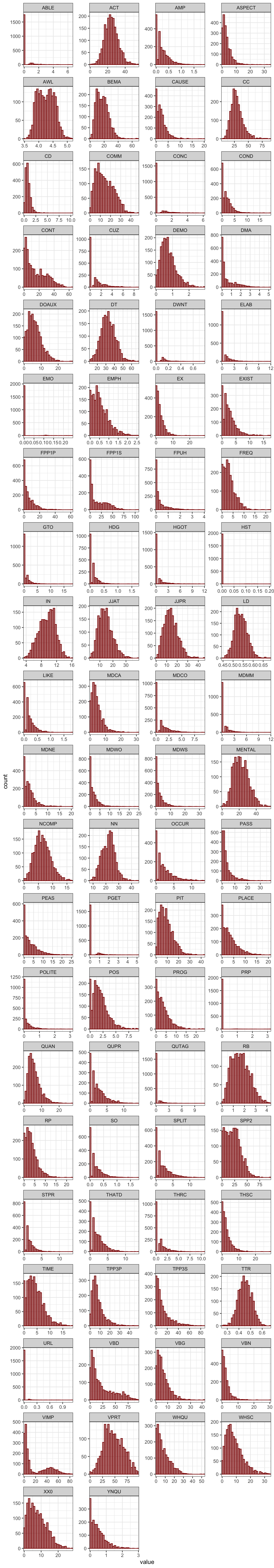
Code
#ggsave(here("plots", "TEC-HistogramPlotsAllVariablesTEC-only.svg"), width = 20, height = 45)E.3.2 Feature removal
A number of features were removed from the dataset as they are not linguistically interpretable. In the case of the TEC, this included the variable CD because numbers spelt out as digits were removed from the textbooks before these were tagged with the MFTE. In addition, the variables LIKE and SO because these are “bin” features included in the output of the MFTE to ensure that the counts for these polysemous words do not inflate other categories due to mistags (Le Foll 2021b).
Whenever linguistically meaningful, very low-frequency features were merged. Finally, features absent from more than third of texts were also excluded. For the analysis intra-textbook register variation, the following linguistic features were excluded from the analysis due to low dispersion:
# Removal of meaningless features:
TxBcounts <- TxBcounts |>
  select(-c(CD, LIKE, SO))

# Function to compute percentage of texts with occurrences meeting a condition
compute_percentage <- function(data, condition, threshold) {
  numeric_data <- Filter(is.numeric, data)
  percentage <- round(colSums(condition[, sapply(numeric_data, is.numeric)])/nrow(data) * 100, 2)
  percentage <- as.data.frame(percentage)
  colnames(percentage) <- "Percentage"
  percentage <- percentage |>
    filter(!is.na(Percentage)) |>
    rownames_to_column() |>
    arrange(Percentage)
  if (!missing(threshold)) {
    percentage <- percentage |>
      filter(Percentage > threshold)
  }
  return(percentage)
}

# Calculate percentage of texts with 0 occurrences of each feature
zero_features <- compute_percentage(TxBcounts, TxBcounts == 0, 66.6)
# zero_features |>
#   kable(col.names = c("Feature", "% texts with zero occurrences"))

# Combine low frequency features into meaningful groups whenever this makes linguistic sense
TxBcounts <- TxBcounts |>
  mutate(JJPR = ABLE + JJPR, ABLE = NULL) |>
  mutate(PASS = PGET + PASS, PGET = NULL)

# Re-calculate percentage of texts with 0 occurrences of each feature
zero_features2 <- compute_percentage(TxBcounts, TxBcounts == 0, 66.6)
zero_features2 |>
kable(col.names = c("Feature", "% texts with zero occurrences"))| Feature | % texts with zero occurrences |
|---|---|
| GTO | 67.07 |
| ELAB | 69.30 |
| MDMM | 70.81 |
| HGOT | 73.75 |
| CONC | 80.48 |
| DWNT | 81.44 |
| QUTAG | 85.99 |
| URL | 96.51 |
| EMO | 97.82 |
| PRP | 98.33 |
| HST | 99.44 |
These feature removal operations resulted in a feature set of 64 linguistic variables.
E.3.3 Identifying potential outlier texts
All normalised frequencies were normalised to identify any potential outlier texts.
TxBzcounts <- TxBcounts |>
  select(-Words) |>
  keep(is.numeric) |>
  scale()

boxplot(TxBzcounts, las = 3, main = "z-scores") # Slow to open!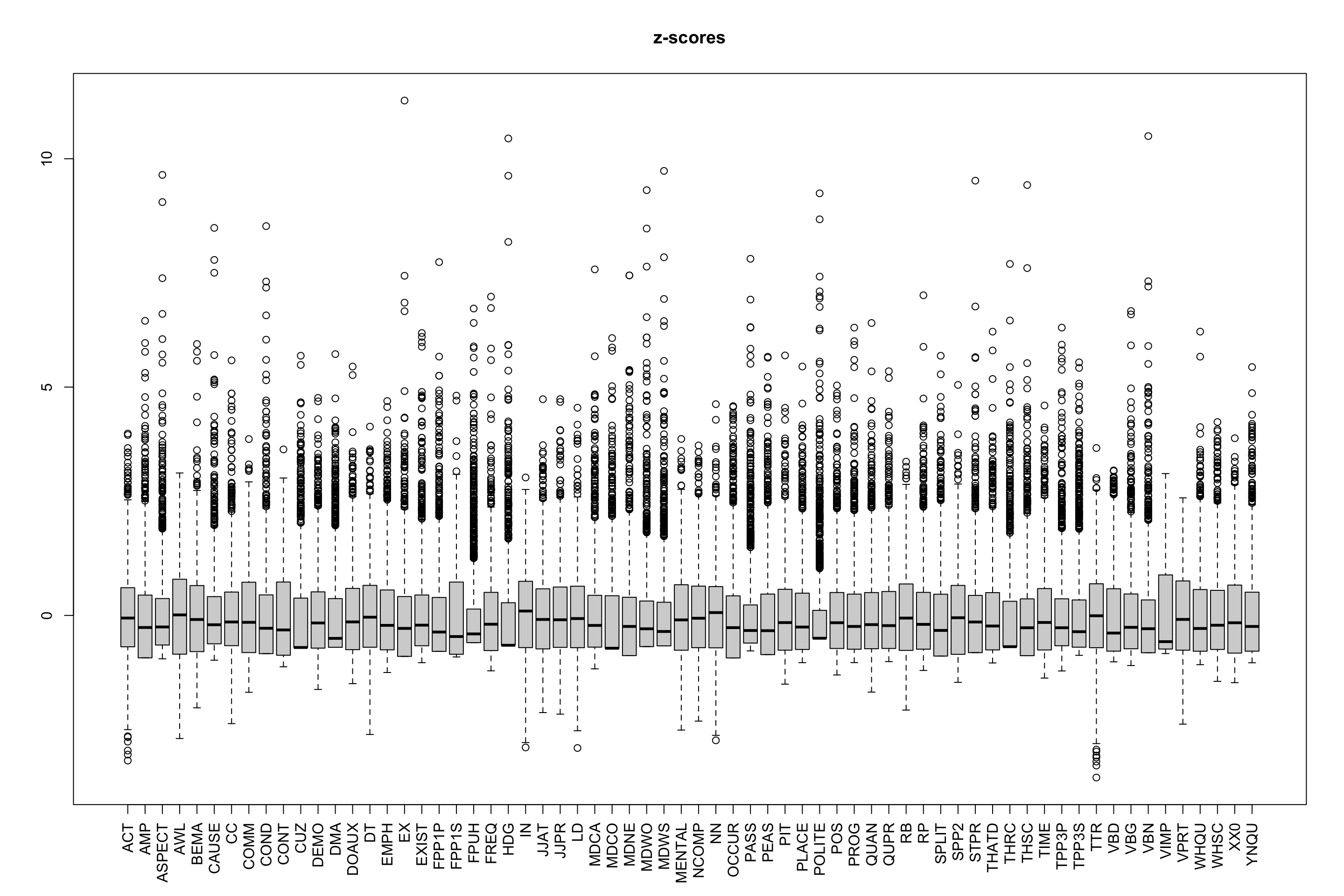
The following outlier texts were identified and excluded in subsequent analyses.
Code
outliers Filename
1 POC_4e_Spoken_0007.txt
2 Solutions_Elementary_Personal_0001.txt
3 NGL_5_Instructional_0018.txt
4 Access_1_Spoken_0011.txt
5 EIM_1_Spoken_0012.txt
6 NGL_4_Spoken_0011.txt
7 Solutions_Intermediate_Plus_Personal_0001.txt
8 Solutions_Elementary_ELF_Spoken_0021.txt
9 NB_2_Informative_0009.txt
10 Solutions_Intermediate_Plus_Spoken_0022.txt
11 Solutions_Intermediate_Instructional_0025.txt
12 Solutions_Pre-Intermediate_Instructional_0024.txt
13 POC_4e_Spoken_0010.txt
14 Solutions_Intermediate_Spoken_0019.txt
15 Access_1_Spoken_0019.txt
16 Solutions_Pre-Intermediate_ELF_Spoken_0005.txtThis resulted in 1,961 TEC texts being included in the model of intra-textbook linguistic variation with the following standardised feature distributions.
Code
TxBzcounts |>
  as.data.frame() |>
  gather() |>  # This function from tidyr converts a selection of variables into two variables: a key and a value. The key contains the names of the original variable and the value the data. This means we can then use the facet_wrap function from ggplot2
  ggplot(aes(value)) +
    theme_bw() +
    facet_wrap(~ key, scales = "free", ncol = 4) +
    scale_x_continuous(expand=c(0,0)) +
geom_histogram(bins = 30, colour= "darkred", fill = "darkred", alpha = 0.5)![]()
Code
#ggsave(here("plots", "TEC-zscores-HistogramsAllVariablesTEC-only.svg"), width = 20, height = 45)E.3.4 Signed log transformation
A signed logarithmic transformation was applied to (further) deskew the feature distributions (Diwersy, Evert & Neumann 2014; Neumann & Evert 2021).
The signed log transformation function was inspired by the SignedLog function proposed in https://cran.r-project.org/web/packages/DataVisualizations/DataVisualizations.pdf
# All features are signed log-transformed (note that this is also what Neumann & Evert 2021 propose)
signed.log <- function(x) {
  sign(x) * log(abs(x) + 1)
  }

TxBzlogcounts <- signed.log(TxBzcounts) # Standardise first, then signed log transform

#saveRDS(TxBzlogcounts, here("data", "processed", "TxBzlogcounts.rds")) # Last saved 6 March 2024
The new feature distributions are visualised below.
Code
TxBzlogcounts |>
  as.data.frame() |>
  gather() |>  # This function from tidyr converts a selection of variables into two variables: a key and a value. The key contains the names of the original variable and the value the data. This means we can then use the facet_wrap function from ggplot2
  ggplot(aes(value, after_stat(density))) +
  theme_bw() +
  facet_wrap(~ key, scales = "free", ncol = 4) +
  scale_x_continuous(expand=c(0,0)) +
  scale_y_continuous(limits = c(0,NA)) +
  geom_histogram(bins = 30, colour= "black", fill = "grey") +
geom_density(colour = "darkred", weight = 2, fill="darkred", alpha = .4)![]()
Code
#ggsave(here("plots", "DensityPlotsAllVariablesSignedLog-TEC-only.svg"), width = 15, height = 49)The following correlation plots serve to illustrate the effect of the variable transformations performed in the above chunks.
Example feature distributions before transformations:
Code
# This is a slightly amended version of the PerformanceAnalytics::chart.Correlation() function. It simply removes the significance stars that are meaningless with this many data points (see commented out lines below)

chart.Correlation.nostars <- function (R, histogram = TRUE, method = c("pearson", "kendall", "spearman"), ...) {
  x = checkData(R, method = "matrix")
  if (missing(method))
    method = method[1]
  panel.cor <- function(x, y, digits = 2, prefix = "", use = "pairwise.complete.obs", method = "pearson", cex.cor, ...) {
    usr <- par("usr")
    on.exit(par(usr))
    par(usr = c(0, 1, 0, 1))
    r <- cor(x, y, use = use, method = method)
    txt <- format(c(r, 0.123456789), digits = digits)[1]
    txt <- paste(prefix, txt, sep = "")
    if (missing(cex.cor))
      cex <- 0.8/strwidth(txt)
    test <- cor.test(as.numeric(x), as.numeric(y), method = method)
    # Signif <- symnum(test$p.value, corr = FALSE, na = FALSE,
    #                  cutpoints = c(0, 0.001, 0.01, 0.05, 0.1, 1), symbols = c("***",
    #                                                                           "**", "*", ".", " "))
    text(0.5, 0.5, txt, cex = cex * (abs(r) + 0.3)/1.3)
    # text(0.8, 0.8, Signif, cex = cex, col = 2)
  }
  f <- function(t) {
    dnorm(t, mean = mean(x), sd = sd.xts(x))
  }
  dotargs <- list(...)
  dotargs$method <- NULL
  rm(method)
  hist.panel = function(x, ... = NULL) {
    par(new = TRUE)
    hist(x, col = "light gray", probability = TRUE,
         axes = FALSE, main = "", breaks = "FD")
    lines(density(x, na.rm = TRUE), col = "red", lwd = 1)
    rug(x)
  }
  if (histogram)
    pairs(x, gap = 0, lower.panel = panel.smooth, upper.panel = panel.cor,
          diag.panel = hist.panel)
  else pairs(x, gap = 0, lower.panel = panel.smooth, upper.panel = panel.cor)
}

# Example plot without any variable transformation
example1 <- TxBcounts |>
  select(NN,PROG,SPLIT,ACT,FPP1S)

#png(here("plots", "CorrChart-TEC-examples-normedcounts.png"), width = 20, height = 20, units = "cm", res = 300)
chart.Correlation.nostars(example1, histogram=TRUE, pch=19)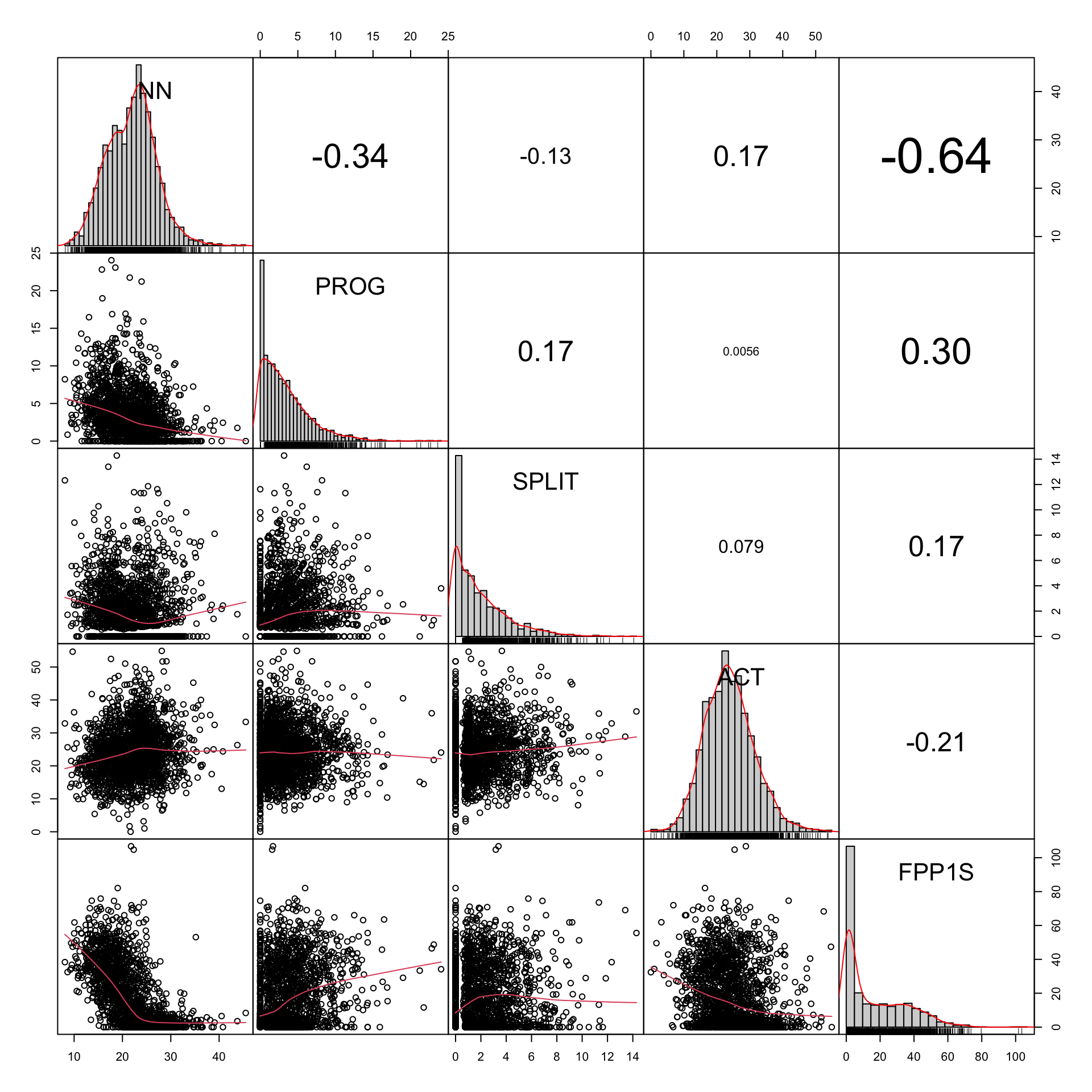
Code
#dev.off()Example feature distributions after transformations:
Code
# Example plot with transformed variables
example2 <- TxBzlogcounts |>
  as.data.frame() |>
  select(NN,PROG,SPLIT,ACT,FPP1S)

#png(here("plots", "CorrChart-TEC-examples-zsignedlogcounts.png"), width = 20, height = 20, units = "cm", res = 300)
chart.Correlation.nostars(example2, histogram=TRUE, pch=19)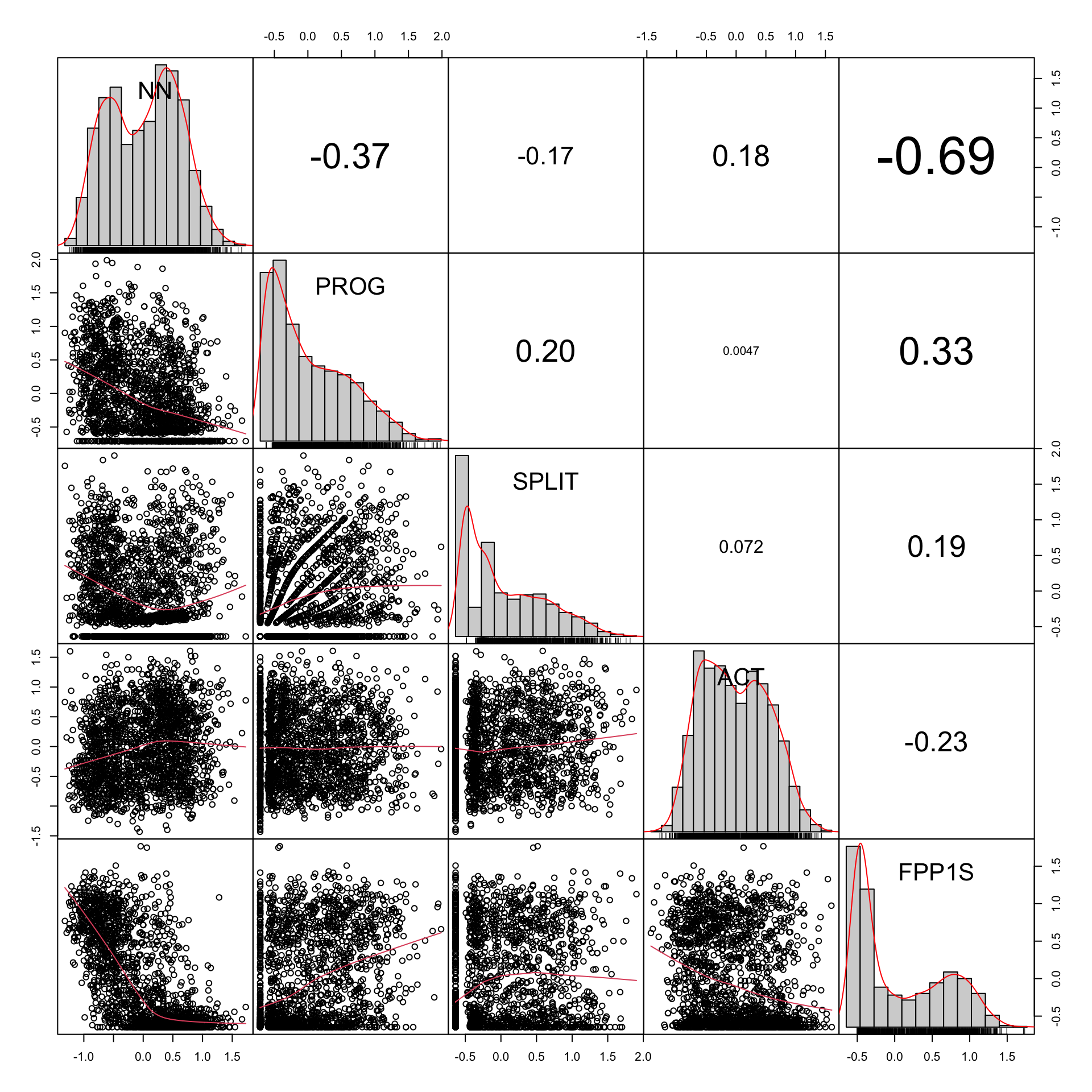
Code
#dev.off()E.3.5 Feature correlations
The correlations of the transformed feature frequencies can be visualised in the form of a heatmap. Negative correlations are rendered in blue, whereas positive ones are in red.
Code
# Simple heatmap in base R (inspired by Stephanie Evert's SIGIL code)
cor.colours <- c(
  hsv(h=2/3, v=1, s=(10:1)/10), # blue = negative correlation
  rgb(1,1,1), # white = no correlation
  hsv(h=0, v=1, s=(1:10/10))) # red = positive correlation

#png(here("plots", "heatmapzlogcounts-TEC-only.png"), width = 30, height= 30, units = "cm", res = 300)
heatmap(cor(TxBzlogcounts),
        symm=TRUE,
        zlim=c(-1,1),
        col=cor.colours,
        margins=c(0,0))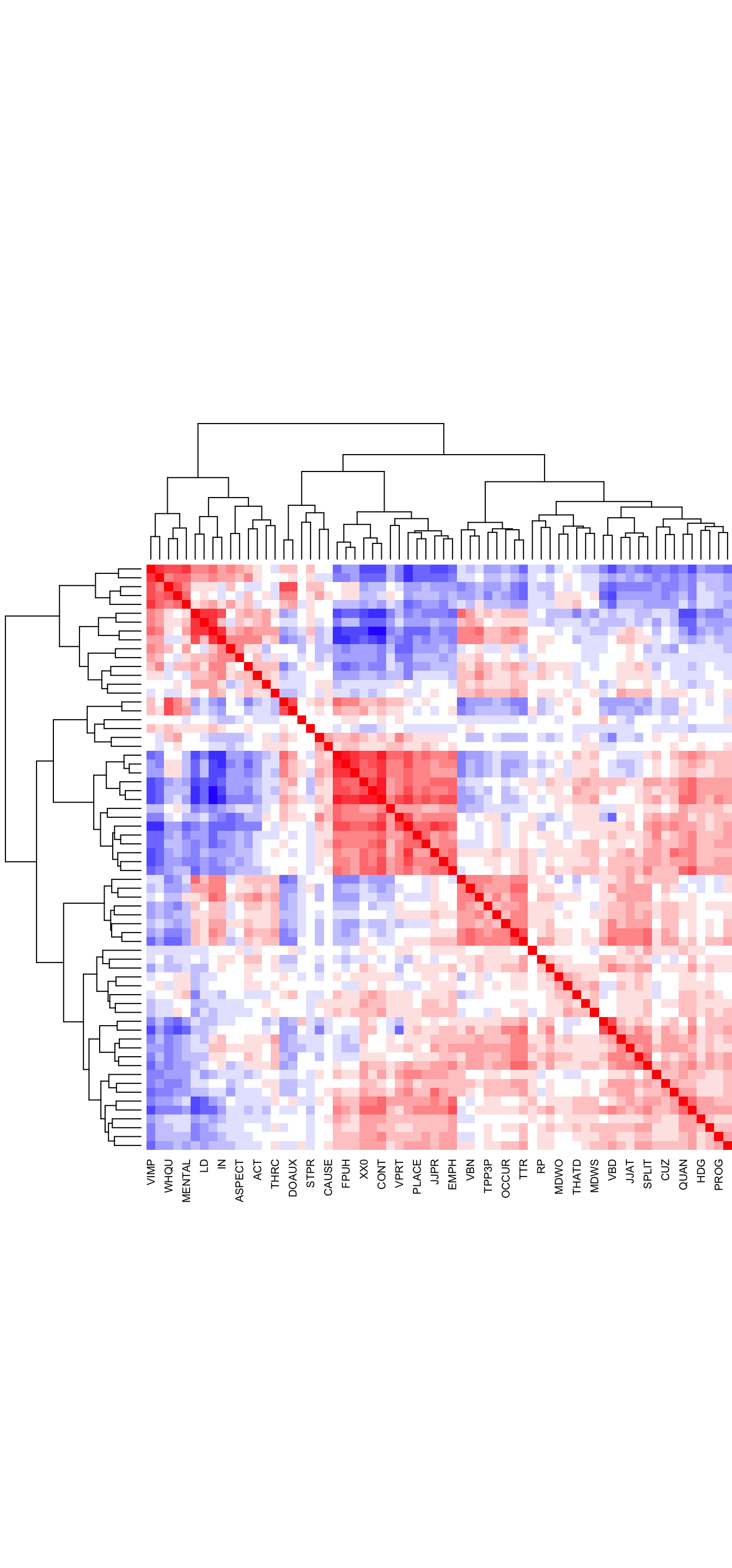
E.4 Composition of TEC texts/files
These figures and tables provide summary statistics on the texts/files of the TEC that were entered in the multi-dimensional model of intra-textbook linguistic variation. In total, the TEC texts entered amounted to 1,693,650 words.
Code
metadata <- TxBcounts |>
  select(Filename, Country, Series, Level, Register, Words) |>
  mutate(Volume = paste(Series, Level)) |>
  mutate(Volume = fct_rev(Volume)) |>
  mutate(Volume = fct_reorder(Volume, as.numeric(Level))) |>
  group_by(Volume) |>
  mutate(wordcount = sum(Words)) |>
  ungroup() |>
  distinct(Volume, .keep_all = TRUE)

# Plot for book
metadata2 <- TxBcounts |>
  select(Country, Series, Level, Register, Words) |>
  mutate(Volume = paste(Series, Level)) |>
  mutate(Volume = fct_rev(Volume)) |>
  #mutate(Volume = fct_reorder(Volume, as.numeric(Level))) |>
  group_by(Volume, Register) |>
  mutate(wordcount = sum(Words)) |>
  ungroup() |>
  distinct(Volume, Register, .keep_all = TRUE)

# This is the palette created above on the basis of the suffrager pakcage (but without needed to install the package)
palette <- c("#BD241E", "#A18A33", "#15274D", "#D54E1E", "#EA7E1E", "#4C4C4C", "#722672", "#F9B921", "#267226")

PlotSp <- metadata2 |>
  filter(Country=="Spain") |>
  #arrange(Volume) |>
  ggplot(aes(x = Volume, y = wordcount, fill = fct_rev(Register))) +
    geom_bar(stat = "identity", position = "stack") +
    coord_flip(expand = FALSE) + # Removes those annoying ticks before each bar label
    theme_minimal() + theme(legend.position = "none") +
    labs(x = "Spain", y = "Cumulative word count") +
    scale_fill_manual(values = palette[c(5,4,3,2,1)],
                      guide = guide_legend(reverse = TRUE))

PlotGer <- metadata2 |>
  filter(Country=="Germany") |>
  #arrange(Volume) |>
  ggplot(aes(x = Volume, y = wordcount, fill = fct_rev(Register))) +
    geom_bar(stat = "identity", position = "stack") +
    coord_flip(expand = FALSE) +
    labs(x = "Germany", y = "") +
    scale_fill_manual(values = palette[c(5,4,3,2,1)], guide = guide_legend(reverse = TRUE)) +
    theme_minimal() + theme(legend.position = "none")

PlotFr <- metadata2 |>
  filter(Country=="France") |>
  #arrange(Volume) |>
  ggplot(aes(x = Volume, y = wordcount, fill = fct_rev(Register))) +
    geom_bar(stat = "identity", position = "stack") +
    coord_flip(expand = FALSE) +
    labs(x = "France", y  = "", fill = "Register subcorpus") +
    scale_fill_manual(values = palette[c(5,4,3,2,1)], guide = guide_legend(reverse = TRUE, legend.hjust = 0)) +
    theme_minimal() + theme(legend.position = "top", legend.justification = "left")

library(patchwork)

PlotFr /
PlotGer /
PlotSp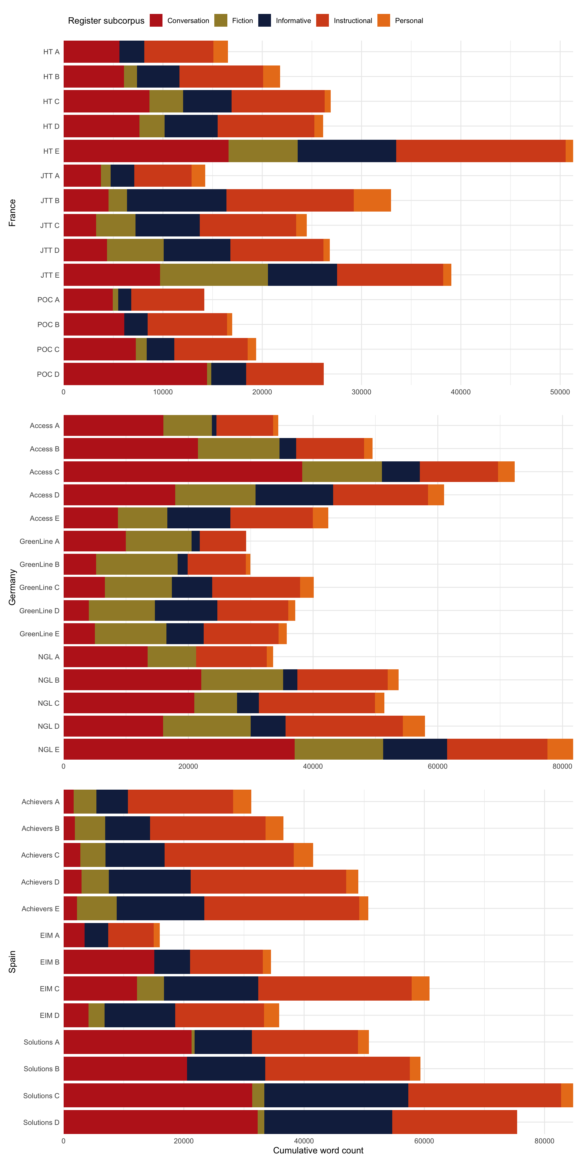
Code
#ggsave(here("plots", "TEC-T_wordcounts_book.svg"), width = 8, height = 12)The following table provides information about the proportion of instructional language featured in each textbook series.
Code
metadataInstr <- TxBcounts |>
  select(Country, Series, Level, Register, Words) |>
  filter(Register=="Instructional") |>
  mutate(Volume = paste(Series, Register)) |>
  mutate(Volume = fct_rev(Volume)) |>
  mutate(Volume = fct_reorder(Volume, as.numeric(Level))) |>
  group_by(Volume, Register) |>
  mutate(InstrWordcount = sum(Words)) |>
  ungroup() |>
  distinct(Volume, .keep_all = TRUE) |>
  select(Series, InstrWordcount)

metaWordcount <- TxBcounts |>
  select(Country, Series, Level, Register, Words) |>
  group_by(Series) |>
  mutate(TECwordcount = sum(Words)) |>
  ungroup() |>
  distinct(Series, .keep_all = TRUE) |>
  select(Series, TECwordcount)

wordcount <- merge(metaWordcount, metadataInstr, by = "Series")

wordcount |>
  mutate(InstrucPercent = InstrWordcount/TECwordcount*100) |>
  arrange(InstrucPercent) |>
  mutate(InstrucPercent = round(InstrucPercent, 2)) |>
  kable(col.names = c("Textbook Series", "Total words", "Instructional words", "% of textbook content"),
        digits = 2,
format.args = list(big.mark = ","))| Textbook Series | Total words | Instructional words | % of textbook content |
|---|---|---|---|
| Access | 259,679 | 60,938 | 23.47 |
| NGL | 278,316 | 79,312 | 28.50 |
| GreenLine | 172,267 | 54,263 | 31.50 |
| Solutions | 270,278 | 87,829 | 32.50 |
| JTT | 137,557 | 48,375 | 35.17 |
| HT | 142,676 | 51,550 | 36.13 |
| POC | 76,714 | 30,548 | 39.82 |
| EIM | 147,185 | 59,928 | 40.72 |
| Achievers | 208,978 | 109,886 | 52.58 |
E.5 Packages used in this script
E.5.1 Package names and versions
R version 4.4.1 (2024-06-14)
Platform: aarch64-apple-darwin20
Running under: macOS Sonoma 14.5

Matrix products: default
BLAS:   /Library/Frameworks/R.framework/Versions/4.4-arm64/Resources/lib/libRblas.0.dylib
LAPACK: /Library/Frameworks/R.framework/Versions/4.4-arm64/Resources/lib/libRlapack.dylib;  LAPACK version 3.12.0

locale:
[1] en_US.UTF-8/en_US.UTF-8/en_US.UTF-8/C/en_US.UTF-8/en_US.UTF-8

time zone: Europe/Madrid
tzcode source: internal

attached base packages:
[1] stats     graphics  grDevices datasets  utils     methods   base

other attached packages:
 [1] lubridate_1.9.3            forcats_1.0.0
 [3] stringr_1.5.1              dplyr_1.1.4
 [5] purrr_1.0.2                readr_2.1.5
 [7] tidyr_1.3.1                tibble_3.2.1
 [9] tidyverse_2.0.0            psych_2.4.6.26
[11] PerformanceAnalytics_2.0.4 xts_0.14.0
[13] zoo_1.8-12                 patchwork_1.2.0
[15] knitr_1.48                 here_1.0.1
[17] DT_0.33                    caret_6.0-94
[19] lattice_0.22-6             ggplot2_3.5.1

loaded via a namespace (and not attached):
 [1] tidyselect_1.2.1     timeDate_4032.109    fastmap_1.2.0
 [4] pROC_1.18.5          digest_0.6.36        rpart_4.1.23
 [7] timechange_0.3.0     lifecycle_1.0.4      survival_3.6-4
[10] magrittr_2.0.3       compiler_4.4.1       rlang_1.1.4
[13] tools_4.4.1          utf8_1.2.4           yaml_2.3.9
[16] data.table_1.15.4    htmlwidgets_1.6.4    mnormt_2.1.1
[19] plyr_1.8.9           withr_3.0.0          nnet_7.3-19
[22] grid_4.4.1           stats4_4.4.1         fansi_1.0.6
[25] colorspace_2.1-0     future_1.33.2        globals_0.16.3
[28] scales_1.3.0         iterators_1.0.14     MASS_7.3-60.2
[31] cli_3.6.3            rmarkdown_2.27       generics_0.1.3
[34] rstudioapi_0.16.0    future.apply_1.11.2  tzdb_0.4.0
[37] reshape2_1.4.4       splines_4.4.1        parallel_4.4.1
[40] BiocManager_1.30.23  vctrs_0.6.5          hardhat_1.4.0
[43] Matrix_1.7-0         jsonlite_1.8.8       hms_1.1.3
[46] listenv_0.9.1        foreach_1.5.2        gower_1.0.1
[49] recipes_1.1.0        glue_1.7.0           parallelly_1.37.1
[52] codetools_0.2-20     stringi_1.8.4        gtable_0.3.5
[55] quadprog_1.5-8       munsell_0.5.1        pillar_1.9.0
[58] htmltools_0.5.8.1    ipred_0.9-15         lava_1.8.0
[61] R6_2.5.1             rprojroot_2.0.4      evaluate_0.24.0
[64] renv_1.0.3           class_7.3-22         Rcpp_1.0.13
[67] nlme_3.1-164         prodlim_2024.06.25   xfun_0.46
[70] pkgconfig_2.0.3      ModelMetrics_1.2.2.2
E.5.2 Package references
[1] G. Grolemund and H. Wickham. “Dates and Times Made Easy with lubridate”. In: Journal of Statistical Software 40.3 (2011), pp. 1-25. https://www.jstatsoft.org/v40/i03/.
[2] M. Kuhn. caret: Classification and Regression Training. R package version 6.0-94. 2023. https://github.com/topepo/caret/.
[3] Kuhn and Max. “Building Predictive Models in R Using the caret Package”. In: Journal of Statistical Software 28.5 (2008), p. 1–26. DOI: 10.18637/jss.v028.i05. https://www.jstatsoft.org/index.php/jss/article/view/v028i05.
[4] K. Müller. here: A Simpler Way to Find Your Files. R package version 1.0.1. 2020. https://here.r-lib.org/.
[5] K. Müller and H. Wickham. tibble: Simple Data Frames. R package version 3.2.1. 2023. https://tibble.tidyverse.org/.
[6] T. L. Pedersen. patchwork: The Composer of Plots. R package version 1.2.0. 2024. https://patchwork.data-imaginist.com.
[7] B. G. Peterson and P. Carl. PerformanceAnalytics: Econometric Tools for Performance and Risk Analysis. R package version 2.0.4. 2020. https://github.com/braverock/PerformanceAnalytics.
[8] R Core Team. R: A Language and Environment for Statistical Computing. R Foundation for Statistical Computing. Vienna, Austria, 2024. https://www.R-project.org/.
[9] W. Revelle. psych: Procedures for Psychological, Psychometric, and Personality Research. R package version 2.4.6.26. 2024. https://personality-project.org/r/psych/.
[10] J. A. Ryan and J. M. Ulrich. xts: eXtensible Time Series. R package version 0.14.0. 2024. https://joshuaulrich.github.io/xts/.
[11] D. Sarkar. Lattice: Multivariate Data Visualization with R. New York: Springer, 2008. ISBN: 978-0-387-75968-5. http://lmdvr.r-forge.r-project.org.
[12] D. Sarkar. lattice: Trellis Graphics for R. R package version 0.22-6. 2024. https://lattice.r-forge.r-project.org/.
[13] V. Spinu, G. Grolemund, and H. Wickham. lubridate: Make Dealing with Dates a Little Easier. R package version 1.9.3. 2023. https://lubridate.tidyverse.org.
[14] H. Wickham. forcats: Tools for Working with Categorical Variables (Factors). R package version 1.0.0. 2023. https://forcats.tidyverse.org/.
[15] H. Wickham. ggplot2: Elegant Graphics for Data Analysis. Springer-Verlag New York, 2016. ISBN: 978-3-319-24277-4. https://ggplot2.tidyverse.org.
[16] H. Wickham. stringr: Simple, Consistent Wrappers for Common String Operations. R package version 1.5.1. 2023. https://stringr.tidyverse.org.
[17] H. Wickham. tidyverse: Easily Install and Load the Tidyverse. R package version 2.0.0. 2023. https://tidyverse.tidyverse.org.
[18] H. Wickham, M. Averick, J. Bryan, et al. “Welcome to the tidyverse”. In: Journal of Open Source Software 4.43 (2019), p. 1686. DOI: 10.21105/joss.01686.
[19] H. Wickham, W. Chang, L. Henry, et al. ggplot2: Create Elegant Data Visualisations Using the Grammar of Graphics. R package version 3.5.1. 2024. https://ggplot2.tidyverse.org.
[20] H. Wickham, R. François, L. Henry, et al. dplyr: A Grammar of Data Manipulation. R package version 1.1.4. 2023. https://dplyr.tidyverse.org.
[21] H. Wickham and L. Henry. purrr: Functional Programming Tools. R package version 1.0.2. 2023. https://purrr.tidyverse.org/.
[22] H. Wickham, J. Hester, and J. Bryan. readr: Read Rectangular Text Data. R package version 2.1.5. 2024. https://readr.tidyverse.org.
[23] H. Wickham, D. Vaughan, and M. Girlich. tidyr: Tidy Messy Data. R package version 1.3.1. 2024. https://tidyr.tidyverse.org.
[24] Y. Xie. Dynamic Documents with R and knitr. 2nd. ISBN 978-1498716963. Boca Raton, Florida: Chapman and Hall/CRC, 2015. https://yihui.org/knitr/.
[25] Y. Xie. “knitr: A Comprehensive Tool for Reproducible Research in R”. In: Implementing Reproducible Computational Research. Ed. by V. Stodden, F. Leisch and R. D. Peng. ISBN 978-1466561595. Chapman and Hall/CRC, 2014.
[26] Y. Xie. knitr: A General-Purpose Package for Dynamic Report Generation in R. R package version 1.48. 2024. https://yihui.org/knitr/.
[27] Y. Xie, J. Cheng, and X. Tan. DT: A Wrapper of the JavaScript Library DataTables. R package version 0.33. 2024. https://github.com/rstudio/DT.
[28] A. Zeileis and G. Grothendieck. “zoo: S3 Infrastructure for Regular and Irregular Time Series”. In: Journal of Statistical Software 14.6 (2005), pp. 1-27. DOI: 10.18637/jss.v014.i06.
[29] A. Zeileis, G. Grothendieck, and J. A. Ryan. zoo: S3 Infrastructure for Regular and Irregular Time Series (Z’s Ordered Observations). R package version 1.8-12. 2023. https://zoo.R-Forge.R-project.org/.