#renv::restore() # Restore the project's dependencies from the lockfile to ensure that same package versions are used as in the original thesis.

library(broom.mixed) # For checking singularity issues
library(car) # For recoding data
library(corrplot) # For the feature correlation matrix
library(cowplot) # For nice plots
library(DT) # To display interactive HTML tables
library(emmeans) # Comparing group means of predicted values
library(GGally) # For ggpairs
library(gridExtra) # For making large faceted plots
library(here) # For ease of sharing
library(knitr) # Loaded to display the tables using the kable() function
library(lme4) # For mixed effects modelling
library(psych) # For various useful stats function, including KMO()
library(scales) # For working with colours
library(sjPlot) # For nice tabular display of regression models
library(tidyverse) # For data wrangling and plotting
library(visreg) # For nice visualisations of model results
select <- dplyr::select
filter <- dplyr::filterAppendix G — Data Preparation for the Model of Textbook English vs. ‘real-world’ English
This script documents the steps taken to pre-process the data extracted from the Textbook English Corpus (TEC) and the three reference corpora that were ultimately entered in the comparative multi-dimensional model of Textbook English as compared to English outside the EFL classroom (Chapter 7).
G.1 Packages required
The following packages must be installed and loaded to process the data.
G.2 Data import from MFTE outputs
The raw data used in this script comes from the matrices of mixed normalised frequencies as output by the MFTE Perl v. 3.1 (Le Foll 2021a).
G.2.1 Spoken BNC2014
Code
SpokenBNC2014 <- read.delim(here("data", "MFTE", "SpokenBNC2014_3.1_normed_complex_counts.tsv"), header = TRUE, stringsAsFactors = TRUE)

SpokenBNC2014$Series <- "Spoken BNC2014"
SpokenBNC2014$Level <- "Ref."
SpokenBNC2014$Country <- "Spoken BNC2014"
SpokenBNC2014$Register <- "Spoken BNC2014"
These normalised frequencies were computed on the basis of my own “John and Jill in Ivybridge” version of the Spoken BNC2014 with added full stops at speaker turns (see Appendix B for details). This corpus comprises of 1,251 texts, all of which were used in the following analyses.
G.2.2 Youth Fiction corpus
Code
YouthFiction <- read.delim(here("data", "MFTE", "YF_sampled_500_3.1_normed_complex_counts.tsv"), header = TRUE, stringsAsFactors = TRUE)

YouthFiction$Series <- "Youth Fiction"
YouthFiction$Level <- "Ref."
YouthFiction$Country <- "Youth Fiction"
YouthFiction$Register <- "Youth Fiction"
These normalised frequencies were computed on the basis of the random samples of approximately 5,000 words of the books of the Youth Fiction corpus (for details of the works included in this corpus, see Appendix B). The sampling procedure is described in Section 4.3.2.4 of the book. This dataset consists of 1,191 files.
G.2.3 Informative Texts for Teens (InfoTeens) corpus
Code
InfoTeen <- read.delim(here("data", "MFTE", "InfoTeen_3.1_normed_complex_counts.tsv"), header = TRUE, stringsAsFactors = TRUE)

# Removes three outlier files which should not have been included in the corpus as they contain exam papers only
InfoTeen <- InfoTeen |>
  filter(Filename!=".DS_Store" & Filename!="Revision_World_GCSE_10529068_wjec-level-law-past-papers.txt" & Filename!="Revision_World_GCSE_10528474_wjec-level-history-past-papers.txt" & Filename!="Revision_World_GCSE_10528472_edexcel-level-history-past-papers.txt")

InfoTeen$Series <- "Info Teens"
InfoTeen$Level <- "Ref."
InfoTeen$Country <- "Info Teens"
InfoTeen$Register <- "Info Teens"
Details of the composition of the Info Teens corpus can be found in Section 4.3.2.5 of the book. The version used in the present study comprises 1,411 texts.
G.3 Merging TEC and reference corpora data
G.3.1 Corpus size
These tables provide some summary statistics about the texts/files whose normalised feature frequencies were entered in the model of Textbook English vs. real-world English described in Chapter 7.
Code
| (Sub)corpus | # texts |
|---|---|
| Textbook Conversation | 593 |
| Textbook Fiction | 285 |
| Info Teens Ref. | 1,411 |
| Textbook Informative | 364 |
| Spoken BNC2014 Ref. | 1,251 |
| Youth Fiction Ref. | 1,191 |
Code
ncounts  |>
  group_by(Register) |>
  summarise(totaltexts = n(),
            totalwords = sum(Words),
            mean = as.integer(mean(Words)),
            sd = as.integer(sd(Words)),
            TTRmean = mean(TTR)) |>
  kable(digits = 2,
        format.args = list(big.mark = ","),
col.names = c("Register", "# texts/files", "# words", "mean # words per text", "SD", "mean TTR"))| Register | # texts/files | # words | mean # words per text | SD | mean TTR |
|---|---|---|---|---|---|
| Conversation | 1,844 | 13,804,196 | 7,486 | 8,690 | 0.40 |
| Fiction | 1,476 | 7,321,747 | 4,960 | 2,022 | 0.49 |
| Informative | 1,775 | 1,436,732 | 809 | 188 | 0.51 |
G.4 Data preparation for PCA
G.4.1 Feature distributions
The distributions of each linguistic features were examined by means of visualisation. As shown below, before transformation, many of the features displayed highly skewed distributions.
Code
#ncounts <- readRDS(here("data", "processed", "counts3Reg.rds"))

ncounts |>
  select(-Words) |>
  keep(is.numeric) |>
  gather() |> # This function from tidyr converts a selection of variables into two variables: a key and a value. The key contains the names of the original variable and the value the data. This means we can then use the facet_wrap function from ggplot2
  ggplot(aes(value, after_stat(density))) +
    theme_bw() +
    facet_wrap(~ key, scales = "free", ncol = 4) +
    scale_x_continuous(expand=c(0,0)) +
    scale_y_continuous(limits = c(0,NA)) +
    geom_histogram(bins = 30, colour= "black", fill = "grey") +
    geom_density(colour = "darkred", weight = 2, fill="darkred", alpha = .4)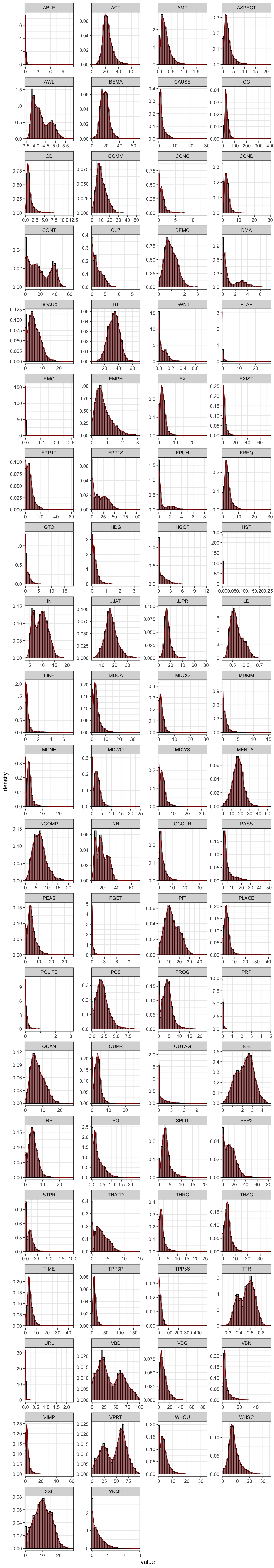
Code
#ggsave(here("plots", "DensityPlotsAllVariables.svg"), width = 15, height = 49)G.4.2 Feature removal
A number of features were removed from the dataset as they are not linguistically interpretable. In the case of the TEC, this included the variable CD because numbers spelt out as digits were removed from the textbooks before these were tagged with the MFTE. In addition, the variables LIKE and SO because these are “bin” features included in the output of the MFTE to ensure that the counts for these polysemous words do not inflate other categories due to mistags (Le Foll 2021b).
Whenever linguistically meaningful, very low-frequency features, features with low MSA or communalities (see chunks below) were merged. Finally, features absent from more than third of texts were also excluded. For the comparative analysis of TEC and the reference corpora, the following linguistic features were excluded from the analysis due to low dispersion:
Code
# Removal of meaningless feature: CD because numbers as digits were mostly removed from the textbooks, LIKE and SO because they are dustbin categories
ncounts <- ncounts |>
  select(-c(CD, LIKE, SO))

# Combine problematic features into meaningful groups whenever this makes linguistic sense
ncounts <- ncounts |>
  mutate(JJPR = JJPR + ABLE, ABLE = NULL) |>
  mutate(PASS = PGET + PASS, PGET = NULL) |>
  mutate(TPP3 = TPP3S + TPP3P, TPP3P = NULL, TPP3S = NULL) |> # Merged due to TTP3P having an individual MSA < 0.5
  mutate(FQTI = FREQ + TIME, FREQ = NULL, TIME = NULL) # Merged due to TIME communality < 0.2 (see below)

# Function to compute percentage of texts with occurrences meeting a condition
compute_percentage <- function(data, condition, threshold) {
  numeric_data <- Filter(is.numeric, data)
  percentage <- round(colSums(condition[, sapply(numeric_data, is.numeric)])/nrow(data) * 100, 2)
  percentage <- as.data.frame(percentage)
  colnames(percentage) <- "Percentage"
  percentage <- percentage |>
    filter(!is.na(Percentage)) |>
    rownames_to_column() |>
    arrange(Percentage)
  if (!missing(threshold)) {
    percentage <- percentage |>
      filter(Percentage > threshold)
  }
  return(percentage)
}

# Calculate percentage of texts with 0 occurrences of each feature
zero_features <- compute_percentage(ncounts, ncounts == 0, 66.6)
zero_features |>
kable(col.names = c("Feature", "% texts with zero occurrences"))| Feature | % texts with zero occurrences |
|---|---|
| PRP | 85.34 |
| URL | 93.03 |
| EMO | 98.98 |
| HST | 99.55 |
These feature removal operations resulted in a feature set of 71 linguistic variables.
G.4.3 Identifying outlier texts
All normalised frequencies were normalised to identify any potential outlier texts.
# First scale the normalised counts (z-standardisation) to be able to compare the various features
zcounts <- ncounts2 |>
  select(-Words) |>
  keep(is.numeric) |>
  scale()

# If necessary, remove any outliers at this stage.
data <- cbind(ncounts2[,1:8], as.data.frame(zcounts))
outliers <- data |>
 filter(if_any(where(is.numeric) & !Words,  .fns = function(x){x > 8}))  |>
  select(Filename, Corpus, Register, Words)
The following outlier texts were identified according to the above conditions and excluded in subsequent analyses.
Code
| Filename | Corpus | Register | # words |
|---|---|---|---|
| POC_4e_Spoken_0007.txt | Textbook.English | Conversation | 750 |
| Solutions_Elementary_ELF_Spoken_0013.txt | Textbook.English | Conversation | 931 |
| EIM_Starter_Informative_0004.txt | Textbook.English | Informative | 534 |
| GreenLine_1_Spoken_0003.txt | Textbook.English | Conversation | 970 |
| Access_1_Spoken_0011.txt | Textbook.English | Conversation | 784 |
| Achievers_B1_Informative_0003.txt | Textbook.English | Informative | 926 |
| EIM_Starter_Spoken_0002.txt | Textbook.English | Conversation | 824 |
| GreenLine_1_Spoken_0008.txt | Textbook.English | Conversation | 876 |
| JTT_3_Informative_0003.txt | Textbook.English | Informative | 699 |
| GreenLine_1_Spoken_0010.txt | Textbook.English | Conversation | 701 |
| EIM_1_Spoken_0012.txt | Textbook.English | Conversation | 640 |
| NGL_1_Spoken_0013.txt | Textbook.English | Conversation | 940 |
| NGL_3_Spoken_0018.txt | Textbook.English | Conversation | 751 |
| Solutions_Intermediate_Spoken_0029.txt | Textbook.English | Conversation | 672 |
| NGL_1_Spoken_0012.txt | Textbook.English | Conversation | 910 |
| GreenLine_1_Spoken_0006.txt | Textbook.English | Conversation | 622 |
| GreenLine_2_Spoken_0004.txt | Textbook.English | Conversation | 1102 |
| Access_2_Spoken_0023.txt | Textbook.English | Conversation | 875 |
| HT_4_Informative_0006.txt | Textbook.English | Informative | 513 |
| Solutions_Intermediate_Informative_0017.txt | Textbook.English | Informative | 816 |
| EIM_1_Spoken_0013.txt | Textbook.English | Conversation | 967 |
| Solutions_Elementary_ELF_Spoken_0021.txt | Textbook.English | Conversation | 846 |
| Solutions_Intermediate_Plus_Spoken_0022.txt | Textbook.English | Conversation | 596 |
| Access_2_Spoken_0028.txt | Textbook.English | Conversation | 813 |
| NGL_1_Spoken_0005.txt | Textbook.English | Conversation | 1020 |
| Solutions_Elementary_ELF_Spoken_0016.txt | Textbook.English | Conversation | 871 |
| Solutions_Pre-Intermediate_ELF_Spoken_0007.txt | Textbook.English | Conversation | 630 |
| Solutions_Intermediate_Informative_0013.txt | Textbook.English | Informative | 770 |
| GreenLine_2_Spoken_0003.txt | Textbook.English | Conversation | 850 |
| HT_4_Spoken_0010.txt | Textbook.English | Conversation | 727 |
| Solutions_Elementary_Informative_0003.txt | Textbook.English | Informative | 1051 |
| Access_2_Informative_0001.txt | Textbook.English | Informative | 655 |
| Solutions_Elementary_Informative_0010.txt | Textbook.English | Informative | 708 |
| GreenLine_1_Informative_0001.txt | Textbook.English | Informative | 731 |
| Access_2_Spoken_0002.txt | Textbook.English | Conversation | 572 |
| Solutions_Intermediate_Spoken_0019.txt | Textbook.English | Conversation | 1024 |
| Access_3_Informative_0003.txt | Textbook.English | Informative | 1000 |
| Access_1_Spoken_0019.txt | Textbook.English | Conversation | 701 |
| Access_2_Spoken_0013.txt | Textbook.English | Conversation | 981 |
| Solutions_Intermediate_Plus_Informative_0014.txt | Textbook.English | Informative | 537 |
| Revision_World_GCSE_10525362_literary-terms.txt | Informative.Teens | Informative | 790 |
| Revision_World_GCSE_10528697_p6-physics-radioactive-materials.txt | Informative.Teens | Informative | 1015 |
| Science_Tech_Kinds_NZ_10382383_math.txt | Informative.Teens | Informative | 522 |
| Science_for_students_10064820_scientists-say-metabolism.txt | Informative.Teens | Informative | 895 |
| Science_Tech_Kinds_NZ_10382388_recycling.txt | Informative.Teens | Informative | 666 |
| History_Kids_BBC_10404337_go_furthers.txt | Informative.Teens | Informative | 620 |
| Science_Tech_Kinds_NZ_10382391_sports.txt | Informative.Teens | Informative | 657 |
| Teen_Kids_News_10402607_so-you-want-to-be-an-archivist.txt | Informative.Teens | Informative | 763 |
| Science_Tech_Kinds_NZ_10382234_biology.txt | Informative.Teens | Informative | 843 |
| Science_Tech_Kinds_NZ_10382372_astronomy.txt | Informative.Teens | Informative | 900 |
| Dogo_News_file10060404_banana-plant-extract-may-be-the-key-to-slower-melting-ice-cream.txt | Informative.Teens | Informative | 611 |
| Science_Tech_Kinds_NZ_10382667_countries.txt | Informative.Teens | Informative | 717 |
| Quatr_us_file10390777_quick-summary-geological-erashtm.txt | Informative.Teens | Informative | 643 |
| Science_Tech_Kinds_NZ_10382873_physics.txt | Informative.Teens | Informative | 722 |
| Science_Tech_Kinds_NZ_10382382_light.txt | Informative.Teens | Informative | 639 |
| Factmonster_10053687_august-13.txt | Informative.Teens | Informative | 523 |
| Revision_World_GCSE_10526703_limited-companies.txt | Informative.Teens | Informative | 714 |
| Revision_World_GCSE_10529637_transition-metals.txt | Informative.Teens | Informative | 787 |
| Quatr_us_10390856_early-african-historyhtm.txt | Informative.Teens | Informative | 1136 |
| History_Kids_BBC_10401873_ff6_sicilylandingss.txt | Informative.Teens | Informative | 813 |
| Quatr_us_10394250_harappan.txt | Informative.Teens | Informative | 651 |
| Ducksters_10398301_iraqphp.txt | Informative.Teens | Informative | 657 |
| History_Kids_BBC_10403171_death_sakkara_gallery_04s.txt | Informative.Teens | Informative | 844 |
| Revision_World_GCSE_10528246_agricultural-change.txt | Informative.Teens | Informative | 789 |
| Revision_World_GCSE_10528086_uk-government-judiciary.txt | Informative.Teens | Informative | 1019 |
| Revision_World_GCSE_10529794_definitions.txt | Informative.Teens | Informative | 904 |
| Encyclopedia_Kinds_au_10085347_Nobel_Prize_in_Chemistry.txt | Informative.Teens | Informative | 598 |
| Science_for_students_10064875_questions-big-melt-earths-ice-sheets-are-under-attack.txt | Informative.Teens | Informative | 685 |
| Teen_Kids_News_10403301_golden-globe-winners-2019-the-complete-list.txt | Informative.Teens | Informative | 800 |
| Science_Tech_Kinds_NZ_10382201_projects.txt | Informative.Teens | Informative | 947 |
| Revision_World_GCSE_10529753_probability.txt | Informative.Teens | Informative | 816 |
| Encyclopedia_Kinds_au_10085531_Complex_analysis.txt | Informative.Teens | Informative | 735 |
| History_Kids_BBC_10401890_ff7_ddays.txt | Informative.Teens | Informative | 759 |
| History_Kids_BBC_10403434s.txt | Informative.Teens | Informative | 732 |
| History_Kids_BBC_10401872_ff6_italys.txt | Informative.Teens | Informative | 786 |
| Science_Tech_Kinds_NZ_10382371_amazing.txt | Informative.Teens | Informative | 629 |
| Quatr_us_10391129_athabascan.txt | Informative.Teens | Informative | 637 |
| Encyclopedia_Kinds_au_10085355_20th_century.txt | Informative.Teens | Informative | 864 |
| Dogo_News_10060755_luxury-space-hotel-promises-guests-a-truly-out-of-this-world-vacation.txt | Informative.Teens | Informative | 722 |
| Revision_World_GCSE_10528072_nationalism-practice.txt | Informative.Teens | Informative | 776 |
| Quatr_us_10390861_quatr-us-privacy-policyhtm.txt | Informative.Teens | Informative | 960 |
| History_Kids_BBC_10401909_ff7_bulges.txt | Informative.Teens | Informative | 732 |
| History_kids_10381259_timeline-of-mesopotamia.txt | Informative.Teens | Informative | 768 |
| Revision_World_GCSE_10528123_gender-written-textual-analysis-framework.txt | Informative.Teens | Informative | 905 |
| Science_Tech_Kinds_NZ_10386406_floods.txt | Informative.Teens | Informative | 580 |
| Revision_World_GCSE_10529693_advantages.txt | Informative.Teens | Informative | 782 |
| Science_Tech_Kinds_NZ_10382378_geography.txt | Informative.Teens | Informative | 761 |
| Science_Tech_Kinds_NZ_10382374_earth.txt | Informative.Teens | Informative | 726 |
| Science_for_students_10066286_watering-plants-wastewater-can-spread-germs.txt | Informative.Teens | Informative | 836 |
| Science_Tech_Kinds_NZ_10382393_water.txt | Informative.Teens | Informative | 856 |
| World_Dteen_10406069_website_policies.txt | Informative.Teens | Informative | 995 |
| Science_Tech_Kinds_NZ_10382384_metals.txt | Informative.Teens | Informative | 669 |
| Dogo_News_10062028_puppy-bowl-14-promises-viewers-a-paw-some-time-on-super-bowl-sunday.txt | Informative.Teens | Informative | 581 |
| History_Kids_BBC_10404730_go_furthers.txt | Informative.Teens | Informative | 611 |
| Science_Tech_Kinds_NZ_10382385_nature.txt | Informative.Teens | Informative | 722 |
| Science_for_students_10065015_scientists-say-dna-sequencing.txt | Informative.Teens | Informative | 953 |
| Quatr_us_file10390817_conifers-pine-trees-gymnospermshtm.txt | Informative.Teens | Informative | 533 |
| TweenTribute_10051509_it-true-elephants-cant-jump.txt | Informative.Teens | Informative | 790 |
| Revision_World_GCSE_10528494_application-software.txt | Informative.Teens | Informative | 855 |
| Revision_World_GCSE_10529581_different-types-questions-examinations.txt | Informative.Teens | Informative | 742 |
| Dogo_News_10061669_the-chinese-city-of-chengdu-may-soon-be-home-to-multiple-moons.txt | Informative.Teens | Informative | 614 |
| Ducksters_10398306_geography_of_ancient_chinaphp.txt | Informative.Teens | Informative | 638 |
| Science_for_students_10065144_scientists-say-multiverse.txt | Informative.Teens | Informative | 712 |
| Science_Tech_Kinds_NZ_10382211_images.txt | Informative.Teens | Informative | 793 |
| Factmonster_10053754_may-18.txt | Informative.Teens | Informative | 497 |
| World_Dteen_10406047_AboutWORLDteen.txt | Informative.Teens | Informative | 1053 |
| Ducksters_10398078_first_new_dealphp.txt | Informative.Teens | Informative | 649 |
| Revision_World_GCSE_10526926_economies-scale.txt | Informative.Teens | Informative | 621 |
| Factmonster_10053201_september-03.txt | Informative.Teens | Informative | 445 |
| Science_Tech_Kinds_NZ_10387183_calciumcarbonates.txt | Informative.Teens | Informative | 804 |
| Science_Tech_Kinds_NZ_10382380_health.txt | Informative.Teens | Informative | 694 |
| Revision_World_GCSE_10529587_sources-finance.txt | Informative.Teens | Informative | 665 |
| Quatr_us_10393444_fishing.txt | Informative.Teens | Informative | 656 |
| Ducksters_10398315_glossary_and_termsphp.txt | Informative.Teens | Informative | 684 |
| S5AA.txt | Spoken.BNC2014 | Conversation | 1869 |
We check that that outlier texts are not particularly long or short texts by looking at the distribution of text/file length of the outliers.
Code
summary(outliers$Words) Min. 1st Qu. Median Mean 3rd Qu. Max.
445.0 655.5 751.0 773.6 860.0 1869.0 Code
hist(outliers$Words, breaks = 30)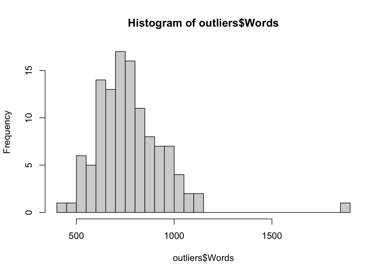
We also check the distribution of outlier texts across the four corpora. The majority come from the Info Teens corpus, though quite a few are also from the TEC.
| (Sub)corpus | # outlier texts |
|---|---|
| Textbook.English | 40 |
| Informative.Teens | 74 |
| Spoken.BNC2014 | 1 |
| Youth.Fiction | 0 |
Code
# Report on the manual check of a sample of these outliers:

# Encyclopedia_Kinds_au_10085347_Nobel_Prize_in_Chemistry.txt is essentially a list of Nobel prize winners but with some additional information. In other words, not a bad representative of the type of texts of the Info Teen corpus.
# Solutions_Elementary_ELF_Spoken_0013 --> Has a lot of "going to" constructions because they are learnt in this chapter but is otherwise a well-formed text.
# Teen_Kids_News_10403972_a-brief-history-of-white-house-weddings --> No issues
# Teen_Kids_News_10403301_golden-globe-winners-2019-the-complete-list --> Similar to the Nobel prize laureates text.
# Revision_World_GCSE_10528123_gender-written-textual-analysis-framework --> Text includes bullet points tokenised as the letter "o" but otherwise a fairly typical informative text.

# Removing the outliers at the request of the reviewers (but comparisons of models including the outliers showed that the results are very similar):
ncounts3 <- ncounts2 |>
  filter(!Filename %in% outliers$Filename)

#saveRDS(ncounts3, here("data", "processed", "ncounts3_3Reg.rds")) # Last saved 6 March 2024
This resulted in 4,980 texts/files being included in the comparative model of Textbook English vs. ‘real-world’ English. These standardised feature frequencies were distributed as follows:
G.4.4 Signed log transformation
A signed logarithmic transformation was applied to (further) deskew the feature distributions (see Diwersy, Evert & Neumann 2014; Neumann & Evert 2021).
The signed log transformation function was inspired by the SignedLog function proposed in https://cran.r-project.org/web/packages/DataVisualizations/DataVisualizations.pdf.
The new feature distributions are visualised below.
Code
zlogcounts |>
  as.data.frame() |>
  gather() |> # This function from tidyr converts a selection of variables into two variables: a key and a value. The key contains the names of the original variable and the value the data. This means we can then use the facet_wrap function from ggplot2
  ggplot(aes(value, after_stat(density))) +
  theme_bw() +
  facet_wrap(~ key, scales = "free", ncol = 4) +
  scale_x_continuous(expand=c(0,0)) +
  scale_y_continuous(limits = c(0,NA)) +
  geom_histogram(bins = 30, colour= "black", fill = "grey") +
geom_density(colour = "darkred", weight = 2, fill="darkred", alpha = .4)![]()
Code
#ggsave(here("plots", "DensityPlotsAllVariablesSignedLog.svg"), width = 15, height = 49)G.4.5 Merging of data for MDA
Code
zlogcounts <- readRDS(here("data", "processed", "zlogcounts_3Reg.rds"))
#nrow(zlogcounts)
#colnames(zlogcounts)

ncounts3 <- readRDS(here("data", "processed", "ncounts3_3Reg.rds"))
#nrow(ncounts3)
#colnames(ncounts3)

data <- cbind(ncounts3[,1:8], as.data.frame(zlogcounts))
#saveRDS(data, here("data", "processed", "datazlogcounts_3Reg.rds")) # Last saved 16 March 2024
The final dataset comprises of 4,980 texts/files, divided as follows:
| (Sub)corpus | # texts/files |
|---|---|
| Textbook Conversation | 565 |
| Textbook Fiction | 285 |
| Info Teens Ref. | 1337 |
| Textbook Informative | 352 |
| Spoken BNC2014 Ref. | 1250 |
| Youth Fiction Ref. | 1191 |
G.5 Testing factorability of data
G.5.1 Visualisation of feature correlations
We begin by visualising the correlations of the transformed feature frequencies using the heatmap function of the stats library. Negative correlations are rendered in blue; positive ones are in red.
Code
# Simple heatmap in base R (inspired by Stephanie Evert's SIGIL code)
cor.colours <- c(
  hsv(h=2/3, v=1, s=(10:1)/10), # blue = negative correlation
  rgb(1,1,1), # white = no correlation
  hsv(h=0, v=1, s=(1:10/10))) # red = positive correlation

#png(here("plots", "heatmapzlogcounts.png"), width = 30, height= 30, units = "cm", res = 300)
heatmap(cor(zlogcounts),
        symm=TRUE,
        zlim=c(-1,1),
        col=cor.colours,
        margins=c(7,7))
Code
#dev.off()G.5.2 Collinearity
As a result of the normalisation unit of finite verb phrases for verb-based features, the present tense (VPRT) and past tense (VBD) variables are correlated to a very high degree:
We therefore remove the least marked of the pair of collinear variables: VPRT.
G.5.3 MSA
The overall MSA value of the dataset is 0.95. The features have the following individual MSA values (ordered from lowest to largest):
   AMP   COMM    POS   TPP3   JJPR  PLACE  SPLIT     DT   JJAT   VIMP   MDCO
  0.67   0.69   0.70   0.74   0.76   0.82   0.83   0.83   0.84   0.84   0.85
    RP     EX   THSC     LD  NCOMP   BEMA   MDWS   FQTI  FPP1P   MDCA    ACT
  0.85   0.85   0.86   0.87   0.88   0.88   0.89   0.89   0.89   0.89   0.89
MENTAL    VBD  FPP1S   MDMM   PEAS   CONC   MDWO   THRC     NN   COND   PROG
  0.91   0.91   0.91   0.91   0.91   0.93   0.93   0.94   0.94   0.95   0.95
    CC   SPP2     RB   DWNT   MDNE   WHSC   CONT   QUPR    XX0  CAUSE   WHQU
  0.95   0.95   0.95   0.95   0.95   0.96   0.96   0.96   0.96   0.96   0.96
   VBG    AWL POLITE   PASS    PIT  DOAUX   ELAB ASPECT    DMA   DEMO    HDG
  0.96   0.96   0.96   0.96   0.97   0.97   0.97   0.97   0.97   0.97   0.97
    IN   FPUH  OCCUR    CUZ   EMPH   YNQU   QUAN    TTR  QUTAG  THATD    VBN
  0.97   0.97   0.97   0.97   0.98   0.98   0.98   0.98   0.98   0.98   0.98
 EXIST   STPR    GTO   HGOT
  0.98   0.99   0.99   0.99
We aim to remove features with an individual MSA < 0.5. All features have individual MSAs of > 0.5 (but only because TPP3P was merged into a broader category in an earlier chunk).
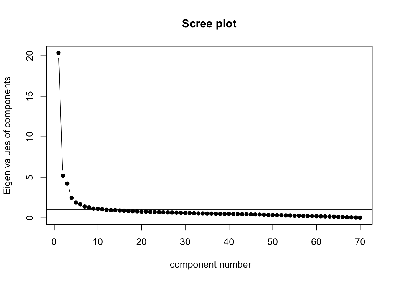
G.5.4 Scree plot
Six components were originally retained on the basis of the following screeplot, though only the first four were found to be interpretable and were therefore included in the model.
G.5.5 Communalities
If features with final communalities of < 0.2 are removed, TIME would have to be removed. TIME was therefore merged with FREQ in an earlier chunk so that now all features have final communalities of > 0.2 (note that this is a very generous threshold!).
  DWNT   STPR   CONC   FQTI    POS ASPECT   MDNE  FPP1P   PROG   MDCO   MDMM
  0.22   0.23   0.23   0.23   0.24   0.25   0.27   0.28   0.29   0.32   0.32
  MDWO  SPLIT   MDWS   PEAS   QUPR    AMP  PLACE    HDG   COMM  CAUSE     EX
  0.32   0.33   0.34   0.35   0.35   0.35   0.37   0.38   0.38   0.38   0.38
  THSC  OCCUR   WHSC   THRC   JJAT   COND MENTAL    ACT   VIMP   ELAB  EXIST
  0.40   0.40   0.42   0.43   0.44   0.44   0.45   0.45   0.46   0.46   0.46
  JJPR  NCOMP     RP    GTO   DEMO   MDCA POLITE    CUZ     CC   WHQU   TPP3
  0.46   0.48   0.49   0.50   0.50   0.52   0.52   0.53   0.57   0.58   0.58
   VBG  THATD    PIT   BEMA  FPP1S     DT   HGOT     RB    VBN  QUTAG   EMPH
  0.60   0.60   0.61   0.61   0.61   0.61   0.62   0.62   0.64   0.64   0.64
  PASS    XX0   QUAN   SPP2  DOAUX    TTR   YNQU    VBD     LD   FPUH     IN
  0.65   0.65   0.67   0.68   0.69   0.71   0.74   0.78   0.81   0.83   0.86
  CONT    DMA    AWL     NN
  0.89   0.89   0.91   0.93
Code
#saveRDS(data, here("data", "processed", "dataforPCA.rds")) # Last saved on 6 March 2024The final dataset entered in the analysis described in Chapter 7 therefore comprises 4,980 texts/files, each with logged standardised normalised frequencies for 70 linguistic features.
G.6 Packages used in this script
G.6.1 Package names and versions
R version 4.4.1 (2024-06-14)
Platform: aarch64-apple-darwin20
Running under: macOS Sonoma 14.5

Matrix products: default
BLAS:   /Library/Frameworks/R.framework/Versions/4.4-arm64/Resources/lib/libRblas.0.dylib
LAPACK: /Library/Frameworks/R.framework/Versions/4.4-arm64/Resources/lib/libRlapack.dylib;  LAPACK version 3.12.0

locale:
[1] en_US.UTF-8/en_US.UTF-8/en_US.UTF-8/C/en_US.UTF-8/en_US.UTF-8

time zone: Europe/Madrid
tzcode source: internal

attached base packages:
[1] stats     graphics  grDevices datasets  utils     methods   base

other attached packages:
 [1] DT_0.33             visreg_2.7.0        lubridate_1.9.3
 [4] forcats_1.0.0       stringr_1.5.1       dplyr_1.1.4
 [7] purrr_1.0.2         readr_2.1.5         tidyr_1.3.1
[10] tibble_3.2.1        tidyverse_2.0.0     sjPlot_2.8.16
[13] scales_1.3.0        psych_2.4.6.26      lme4_1.1-35.5
[16] Matrix_1.7-0        knitr_1.48          here_1.0.1
[19] gridExtra_2.3       GGally_2.2.1        ggplot2_3.5.1
[22] emmeans_1.10.3      cowplot_1.1.3       corrplot_0.92
[25] car_3.1-2           carData_3.0-5       broom.mixed_0.2.9.5

loaded via a namespace (and not attached):
 [1] tidyselect_1.2.1    sjlabelled_1.2.0    fastmap_1.2.0
 [4] sjstats_0.19.0      digest_0.6.36       timechange_0.3.0
 [7] estimability_1.5.1  lifecycle_1.0.4     magrittr_2.0.3
[10] compiler_4.4.1      rlang_1.1.4         tools_4.4.1
[13] utf8_1.2.4          yaml_2.3.9          htmlwidgets_1.6.4
[16] mnormt_2.1.1        plyr_1.8.9          RColorBrewer_1.1-3
[19] abind_1.4-5         withr_3.0.0         grid_4.4.1
[22] datawizard_0.12.1   fansi_1.0.6         xtable_1.8-4
[25] colorspace_2.1-0    future_1.33.2       globals_0.16.3
[28] MASS_7.3-60.2       insight_0.20.2      cli_3.6.3
[31] mvtnorm_1.2-5       rmarkdown_2.27      generics_0.1.3
[34] rstudioapi_0.16.0   performance_0.12.2  tzdb_0.4.0
[37] minqa_1.2.7         splines_4.4.1       parallel_4.4.1
[40] BiocManager_1.30.23 vctrs_0.6.5         boot_1.3-30
[43] jsonlite_1.8.8      hms_1.1.3           listenv_0.9.1
[46] glue_1.7.0          parallelly_1.37.1   nloptr_2.1.1
[49] ggstats_0.6.0       codetools_0.2-20    stringi_1.8.4
[52] gtable_0.3.5        ggeffects_1.7.0     munsell_0.5.1
[55] furrr_0.3.1         pillar_1.9.0        htmltools_0.5.8.1
[58] R6_2.5.1            rprojroot_2.0.4     evaluate_0.24.0
[61] lattice_0.22-6      backports_1.5.0     broom_1.0.6
[64] renv_1.0.3          Rcpp_1.0.13         coda_0.19-4.1
[67] nlme_3.1-164        xfun_0.46           sjmisc_2.8.10
[70] pkgconfig_2.0.3
G.6.2 Package references
[1] B. Auguie. gridExtra: Miscellaneous Functions for “Grid” Graphics. R package version 2.3. 2017.
[2] D. Bates, M. Mächler, B. Bolker, et al. “Fitting Linear Mixed-Effects Models Using lme4”. In: Journal of Statistical Software 67.1 (2015), pp. 1-48. DOI: 10.18637/jss.v067.i01.
[3] D. Bates, M. Maechler, B. Bolker, et al. lme4: Linear Mixed-Effects Models using Eigen and S4. R package version 1.1-35.5. 2024. https://github.com/lme4/lme4/.
[4] D. Bates, M. Maechler, and M. Jagan. Matrix: Sparse and Dense Matrix Classes and Methods. R package version 1.7-0. 2024. https://Matrix.R-forge.R-project.org.
[5] B. Bolker and D. Robinson. broom.mixed: Tidying Methods for Mixed Models. R package version 0.2.9.5. 2024. https://github.com/bbolker/broom.mixed.
[6] P. Breheny and W. Burchett. visreg: Visualization of Regression Models. R package version 2.7.0. 2020. http://pbreheny.github.io/visreg.
[7] P. Breheny and W. Burchett. “Visualization of Regression Models Using visreg”. In: The R Journal 9.2 (2017), pp. 56-71.
[8] J. Fox and S. Weisberg. An R Companion to Applied Regression. Third. Thousand Oaks CA: Sage, 2019. https://socialsciences.mcmaster.ca/jfox/Books/Companion/.
[9] J. Fox, S. Weisberg, and B. Price. car: Companion to Applied Regression. R package version 3.1-2. 2023. https://r-forge.r-project.org/projects/car/.
[10] J. Fox, S. Weisberg, and B. Price. carData: Companion to Applied Regression Data Sets. R package version 3.0-5. 2022. https://r-forge.r-project.org/projects/car/.
[11] G. Grolemund and H. Wickham. “Dates and Times Made Easy with lubridate”. In: Journal of Statistical Software 40.3 (2011), pp. 1-25. https://www.jstatsoft.org/v40/i03/.
[12] R. V. Lenth. emmeans: Estimated Marginal Means, aka Least-Squares Means. R package version 1.10.3. 2024. https://rvlenth.github.io/emmeans/.
[13] D. Lüdecke. sjPlot: Data Visualization for Statistics in Social Science. R package version 2.8.16. 2024. https://strengejacke.github.io/sjPlot/.
[14] K. Müller. here: A Simpler Way to Find Your Files. R package version 1.0.1. 2020. https://here.r-lib.org/.
[15] K. Müller and H. Wickham. tibble: Simple Data Frames. R package version 3.2.1. 2023. https://tibble.tidyverse.org/.
[16] R Core Team. R: A Language and Environment for Statistical Computing. R Foundation for Statistical Computing. Vienna, Austria, 2024. https://www.R-project.org/.
[17] W. Revelle. psych: Procedures for Psychological, Psychometric, and Personality Research. R package version 2.4.6.26. 2024. https://personality-project.org/r/psych/.
[18] B. Schloerke, D. Cook, J. Larmarange, et al. GGally: Extension to ggplot2. R package version 2.2.1. 2024. https://ggobi.github.io/ggally/.
[19] V. Spinu, G. Grolemund, and H. Wickham. lubridate: Make Dealing with Dates a Little Easier. R package version 1.9.3. 2023. https://lubridate.tidyverse.org.
[20] T. Wei and V. Simko. corrplot: Visualization of a Correlation Matrix. R package version 0.92. 2021. https://github.com/taiyun/corrplot.
[21] T. Wei and V. Simko. R package ‘corrplot’: Visualization of a Correlation Matrix. (Version 0.92). 2021. https://github.com/taiyun/corrplot.
[22] H. Wickham. forcats: Tools for Working with Categorical Variables (Factors). R package version 1.0.0. 2023. https://forcats.tidyverse.org/.
[23] H. Wickham. ggplot2: Elegant Graphics for Data Analysis. Springer-Verlag New York, 2016. ISBN: 978-3-319-24277-4. https://ggplot2.tidyverse.org.
[24] H. Wickham. stringr: Simple, Consistent Wrappers for Common String Operations. R package version 1.5.1. 2023. https://stringr.tidyverse.org.
[25] H. Wickham. tidyverse: Easily Install and Load the Tidyverse. R package version 2.0.0. 2023. https://tidyverse.tidyverse.org.
[26] H. Wickham, M. Averick, J. Bryan, et al. “Welcome to the tidyverse”. In: Journal of Open Source Software 4.43 (2019), p. 1686. DOI: 10.21105/joss.01686.
[27] H. Wickham, W. Chang, L. Henry, et al. ggplot2: Create Elegant Data Visualisations Using the Grammar of Graphics. R package version 3.5.1. 2024. https://ggplot2.tidyverse.org.
[28] H. Wickham, R. François, L. Henry, et al. dplyr: A Grammar of Data Manipulation. R package version 1.1.4. 2023. https://dplyr.tidyverse.org.
[29] H. Wickham and L. Henry. purrr: Functional Programming Tools. R package version 1.0.2. 2023. https://purrr.tidyverse.org/.
[30] H. Wickham, J. Hester, and J. Bryan. readr: Read Rectangular Text Data. R package version 2.1.5. 2024. https://readr.tidyverse.org.
[31] H. Wickham, T. L. Pedersen, and D. Seidel. scales: Scale Functions for Visualization. R package version 1.3.0. 2023. https://scales.r-lib.org.
[32] H. Wickham, D. Vaughan, and M. Girlich. tidyr: Tidy Messy Data. R package version 1.3.1. 2024. https://tidyr.tidyverse.org.
[33] C. O. Wilke. cowplot: Streamlined Plot Theme and Plot Annotations for ggplot2. R package version 1.1.3. 2024. https://wilkelab.org/cowplot/.
[34] Y. Xie. Dynamic Documents with R and knitr. 2nd. ISBN 978-1498716963. Boca Raton, Florida: Chapman and Hall/CRC, 2015. https://yihui.org/knitr/.
[35] Y. Xie. “knitr: A Comprehensive Tool for Reproducible Research in R”. In: Implementing Reproducible Computational Research. Ed. by V. Stodden, F. Leisch and R. D. Peng. ISBN 978-1466561595. Chapman and Hall/CRC, 2014.
[36] Y. Xie. knitr: A General-Purpose Package for Dynamic Report Generation in R. R package version 1.48. 2024. https://yihui.org/knitr/.
[37] Y. Xie, J. Cheng, and X. Tan. DT: A Wrapper of the JavaScript Library DataTables. R package version 0.33. 2024. https://github.com/rstudio/DT.