Appendix H — Data Analysis for the Model of Textbook English vs. ‘real-world’ English

Last modifications on this page

January 24, 2025

This script documents the analysis of data from the TEC and reference corpus data (as pre-processed in Appendix F) to arrive at the multi-dimensional model of Textbook Englisch vs. ‘real-world’ English described in Chapter 7. It generates all of the statistics and plots included in the book, as well as many others that were used in the analysis, but were not included in the book for reasons of space.

H.1 Packages required

The following packages must be installed and loaded to process the data.

#renv::restore() # Restore the project's dependencies from the lockfile to ensure that same package versions are used as in the original thesis.

library(caret) # For its confusion matrix function
library(cowplot) # For its plot themes
library(DescTools) # For 95% CI
library(emmeans) # For the emmeans function
library(factoextra) # For circular graphs of variables
library(gtsummary) # For nice table of summary statistics (optional)
library(gridExtra) # For Fig. 35
library(here) # For dynamic file paths
library(ggthemes) # For theme of factoextra plots
library(knitr) # Loaded to display the tables using the kable() function
library(lme4) # For linear regression modelling
library(patchwork) # To create figures with more than one plot
#library(pca3d) # For 3-D plots (not rendered in exports)
library(PCAtools) # For nice biplots of PCA results
library(psych) # For various useful stats function
library(sjPlot) # For model plots and tables
library(tidyverse) # For data wrangling
library(visreg) # For plots of interaction effects

source(here("R_rainclouds.R")) # For geom_flat_violin rainplots

H.2 Conducting the PCA

We first import the full dataset (see Appendix F for data preparation steps).

The following chunks can be used to perform the MDA on various subsets of the data (see also Section 10.1.1 in the book).

Subset of the data that excludes the lower-level textbooks:

data <- readRDS(here("processed_data", "dataforPCA.rds")) |>
  filter(Level !="A" & Level != "B") |>
  droplevels()
summary(data$Level)

Subset of the data that includes only one Country` subcorpus of the TEC (note that a detailed analysis of the German subcorpus can be found in (Le Foll)):

data <- readRDS(here("processed_data", "dataforPCA.rds")) |>
  #filter(Country != "France" & Country != "Germany") |> # Spain only
  #filter(Country != "France" & Country != "Spain") |> # Germany only
  filter(Country != "Spain" & Country != "Germany") |> # France only
  droplevels()
summary(data$Country)

Random subsets of the data to test the stability of the model proposed in Chapter 7. Re-running this line will generate a new subset of 2/3 of the texts randomly sampled. set.seed(13) was used for the analyses reported on in Section 10.1.1.

set.seed(13) 
data <- readRDS(here("processed_data", "dataforPCA.rds")) |>
  slice_sample(n = 4980*0.6, replace = FALSE)
nrow(data)
data$Filename[1:4]
#Using the set.seed(13), these should be:
#[1] HT_4_Spoken_0009.txt                       
#[2] Solutions_Intermediate_Plus_Spoken_0020.txt
#[3] 141_PRATCHETT1992DW13GODS_4.txt            
#[4] Achievers_B2_Informative_0004.txt

H.3 Plotting PCA results

H.3.1 3D plots

The following chunk can be used to create projections of TEC texts on three dimensions of the model. These plots cannot be rendered in two dimensions and are therefore not generated in the present document. For more information on the pca3d library, see: https://cran.r-project.org/web/packages/pca3d/vignettes/pca3d.pdf.

# Data preparation for 3D plots
colnames(data) # Checking that the features start at the 9th column
pca <- prcomp(data[,9:ncol(data)], scale.=FALSE) # All quantitative variables that contribute to the model
register <- factor(data[,"Register"]) 
corpus <- factor(data[,"Corpus"])
subcorpus <- factor(data[,"Subcorpus"])

library(pca3d)

pca3d(pca, group = subcorpus,
       components = 1:3,
       components = 4:6,
       show.plane=FALSE,
       col = col6,
       shape = shapes6,
       radius = 0.7,
       legend = "right")

snapshotPCA3d(here("plots", "PCA_TxB_3Ref_3Dsnapshot.png"))

# Alternative visualisation, looking at all three Textbook English registers in one colour

pca3d(pca, group = corpus, 
      show.plane=FALSE,
      components = 1:3,
      col = col4,
      shape = shapes4,
      radius = 0.7,
      legend = "right")

H.4 Two-dimensional plots (biplots)

These plots were generated using the PCAtools package, which requires the data to be formatted in a rather unconventional way so it needs to wrangled first.

H.4.1 Data wrangling for PCAtools

Code

# Data wrangling
data2 <- data |> 
  mutate(Source = recode_factor(Corpus, Textbook.English = "Textbook English (TEC)", Informative.Teens = "Reference corpora", Spoken.BNC2014 = "Reference corpora", Youth.Fiction = "Reference corpora")) |> 
  mutate(Corpus = fct_relevel(Subcorpus, "Info Teens Ref.", after = 9)) |>
  relocate(Source, .after = "Corpus") |> 
  droplevels()

# colnames(data2)
data2meta <- data2[,1:9]
rownames(data2meta) <- data2meta$Filename
data2meta <- data2meta |> select(-Filename)
# head(data2meta)
rownames(data2) <- data2$Filename
data2num <- as.data.frame(base::t(data2[,10:ncol(data2)]))
# data2num[1:5,1:5] # Check data frame format is correct by comparing to output of head(data2meta) above

p <- PCAtools::pca(data2num, 
         metadata = data2meta,
         scale = FALSE)

The cumulative proportion of variance in the dataset explained the first four components explain 47.15%.

H.4.2 Pairs plot

This chunk produces a scatterplot matrix of combinations of the four dimensions of the model of Textbook English vs. ‘real-world’ English. Note that the number before the comma on each axis label shows which principal component is plotted on that axis; this is followed by the percentage of the total variance explained by that particular component. The colours correspond to the text registers.

Code

# For five TEC registers
# colkey = c(`Spoken BNC2014 Ref.`="#BD241E", `Info Teens Ref.`="#15274D", `Youth Fiction Ref.`="#267226", `Textbook Fiction`="#A18A33", `Textbook Conversation`="#F9B921", `Textbook Informative` = "#722672", `Textbook Instructional` = "grey", `Textbook Personal` = "black")

# For three TEC registers
# summary(data2$Corpus)
colkey = c(`Spoken BNC2014 Ref.`="#BD241E", `Info Teens Ref.`="#15274D", `Youth Fiction Ref.`="#267226", `Textbook Fiction`="#A18A33", `Textbook Conversation`="#F9B921", `Textbook Informative` = "#722672")

#summary(data2$Source)
#shapekey = c(`Textbook English (TEC)`=6, `Reference corpora`=1)

# summary(data2$Level)
shapekey = c(A=1, B=2, C=6, D=0, E=5, `Ref.`=4)

## Warning: this can be very slow! Open in extra zoomed out window!

#png(here("plots", "PCA_3Ref_pairsplot.png"), width = 12, height= 19, units = "cm", res = 300)
PCAtools::pairsplot(p,
                 triangle = FALSE,
                 components = 1:4,
                 ncol = 2,
                 nrow = 3,
                 pointSize = 0.6,
                 shape = "Level",
                 shapekey = shapekey,
                 lab = NULL, # Otherwise will try to label each data point!
                 colby = "Corpus",
                 legendPosition = "none",
                 margingaps = unit(c(0.2, 0.2, 0.8, 0.2), "cm"),
                 colkey = colkey)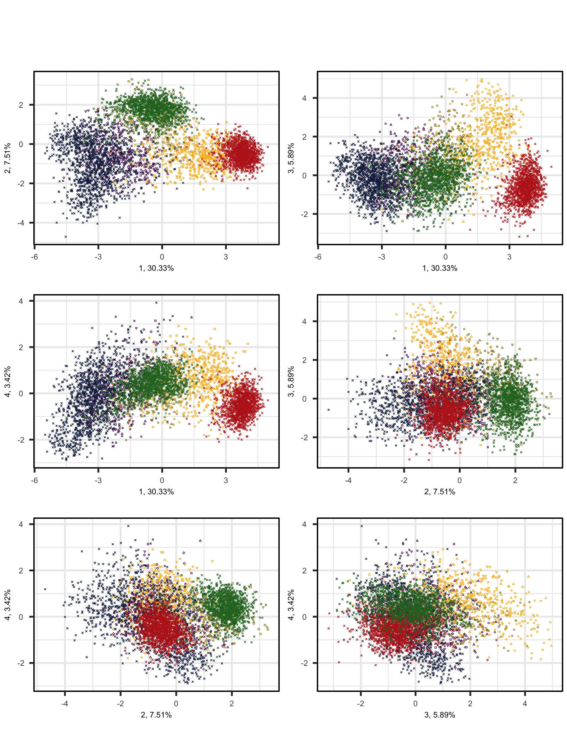

Code

#dev.off()
#ggsave(here("plots", "PCA_TxB_pairsplot.svg"), width = 6, height = 10)
# Note that the legend has to be added manually (it was taken from the biplot code below).

H.4.3 Bi-plots

Biplots are used to more closely examine the position of texts on just two dimensions.

Code

# These settings (with legendPosition = "top") were used to generate the legend for the scatterplot matrix above:
#png(here("plots", "PCA_3Ref_Biplot_PC1_PC2test.png"), width = 40, height= 25, units = "cm", res = 300) 

PCAtools::biplot(p,
                 x = "PC1",
                 y = "PC2",
                 lab = NULL, # Otherwise will try to label each data point!
                 colby = "Corpus",
                 pointSize = 1.3,
                 colkey = colkey,
                 shape = "Level",
                 shapekey = shapekey,
                 xlim = c(min(p$rotated[, "PC1"]), max(p$rotated[, "PC1"])),
                 ylim = c(min(p$rotated[, "PC2"]), max(p$rotated[, "PC2"])),
                 showLoadings = FALSE,
                 ellipse = TRUE,
                 axisLabSize = 18,
                 legendPosition = 'right',
                 legendTitleSize = 18,
                 legendLabSize = 14, 
                 legendIconSize = 5) +
  theme(plot.margin = unit(c(0,0,0,0.2), "cm"))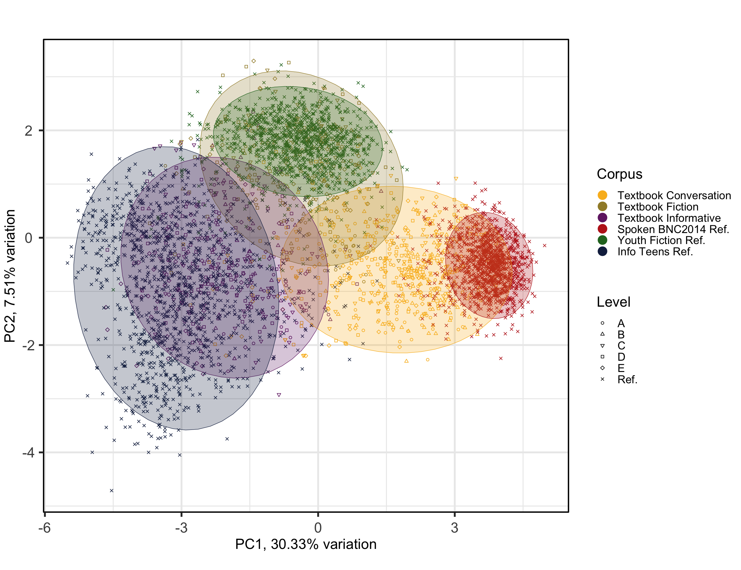

Code

#ggsave(here("plots", "PCA_Ref3TxB_BiplotPC1_PC2.svg"), width = 12, height = 8)

# Biplots to examine components more carefully
PCAtools::biplot(p,
                 x = "PC3",
                 y = "PC4",
                 lab = NULL, # Otherwise will try to label each data point!
                 colby = "Corpus",
                 pointSize = 1.2,
                 colkey = colkey,
                 shape = "Level",
                 shapekey = shapekey,
                 xlim = c(min(p$rotated[, "PC3"]), max(p$rotated[, "PC3"])),
                 ylim = c(min(p$rotated[, "PC4"]), max(p$rotated[, "PC4"])),
                 showLoadings = FALSE,
                 ellipse = TRUE,
                 axisLabSize = 18,
                 legendPosition = 'right',
                 legendTitleSize = 18,
                 legendLabSize = 14, 
                 legendIconSize = 5) +
  theme(plot.margin = unit(c(0,0,0,0.2), "cm"))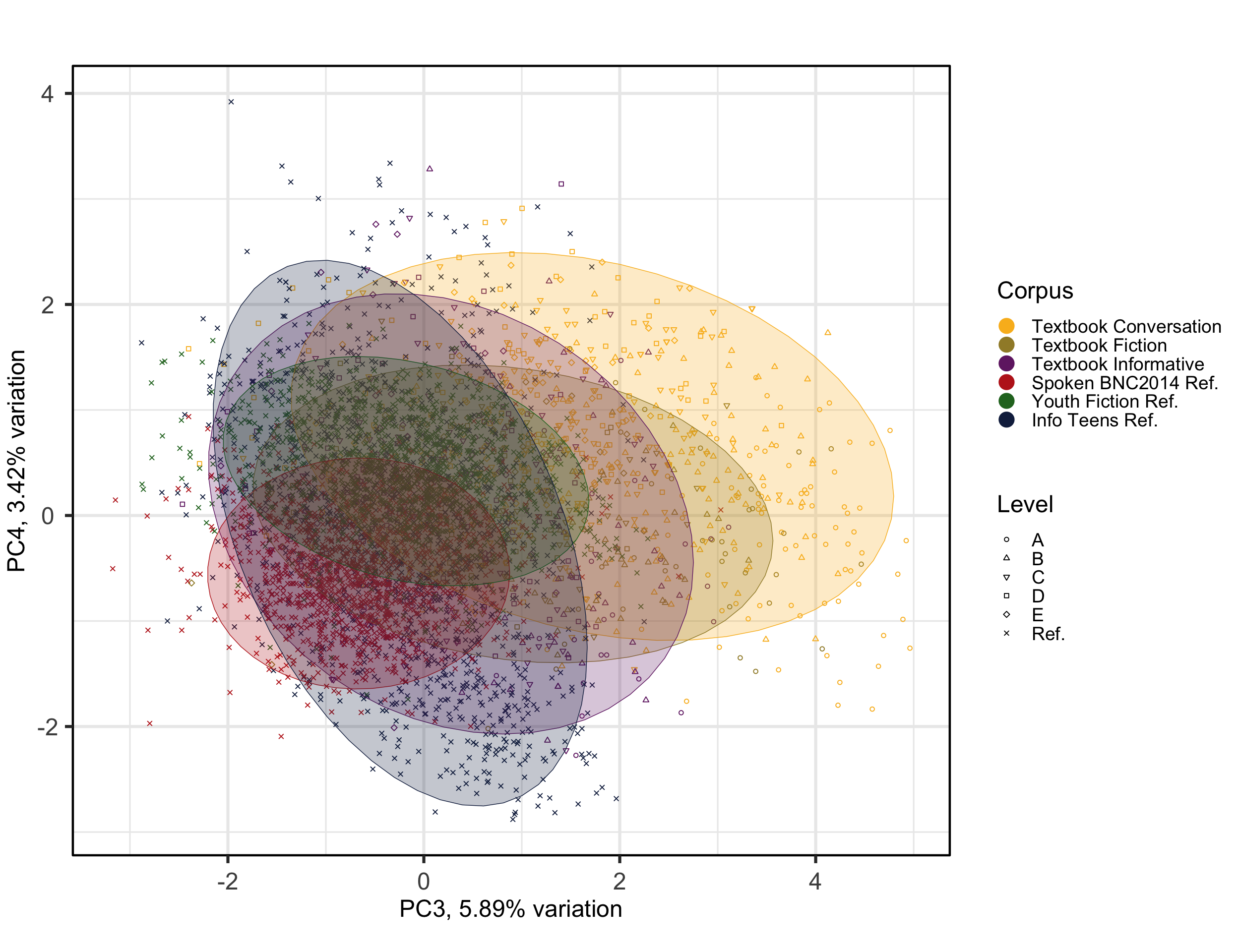

Code

#ggsave(here("plots", "PCA_Ref3TxB_BiplotPC3_PC4.svg"), width = 12, height = 8)

The colours and corresponding ellipses can be used to visualise different clusters and patterns. In the following, we change the colour of the points and the ellipses to represent the texts’ target proficiency levels instead of the register, allowing for a different interpretation of the model.

Code

# Biplot with ellipses for Level rather than Register
colkeyLevels = c(A="#F9B921", B="#A18A33", C="#BD241E", D="#722672", E="#15274D", `Ref. data`= "darkgrey")
shapekeyLevels = c(`Spoken BNC2014 Ref.`=16, `Info Teens Ref.`=17, `Youth Fiction Ref.`=15, `Textbook Fiction`=0, `Textbook Conversation`=1, `Textbook Informative`=2)

PCAtools::biplot(p,
                 x = "PC3",
                 y = "PC4",
                 lab = NULL, # Otherwise will try to label each data point!
                 colby = "Level",
                 pointSize = 1.3,
                 colkey = colkeyLevels,
                 shape = "Corpus",
                 shapekey = shapekeyLevels,
                 xlim = c(min(p$rotated[, "PC3"]), max(p$rotated[, "PC3"])),
                 ylim = c(min(p$rotated[, "PC4"]), max(p$rotated[, "PC4"])),
                 showLoadings = FALSE,
                 ellipse = TRUE,
                 axisLabSize = 18,
                 legendPosition = 'right',
                 legendTitleSize = 18,
                 legendLabSize = 14, 
                 legendIconSize = 5) +
  theme(plot.margin = unit(c(0,0,0,0.2), "cm"))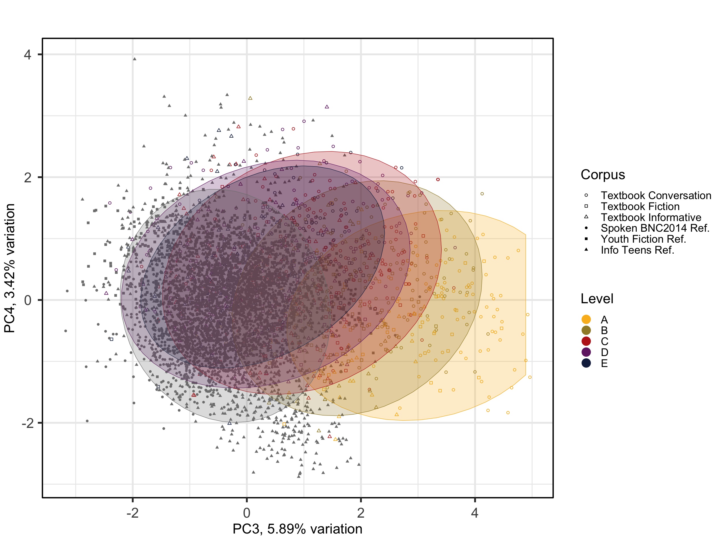

Code

#ggsave(here("plots", "PCA_Ref3TxB_BiplotPC3_PC4_levels.svg"), width = 12, height = 8)

H.5 Feature contributions (loadings) on each component

Code

pca <- prcomp(data[,9:ncol(data)], scale.=FALSE) # All quantitative variables to be included in the model

# The rotated data that represents the observations / samples is stored in rotated, while the variable loadings are stored in loadings
loadings <- as.data.frame(pca$rotation[,1:4])

# Table of loadings with no minimum threshold applied
loadings |> 
  round(2) |> 
  kable()

	PC1	PC2	PC3	PC4
ACT	-0.10	0.01	-0.01	0.12
AMP	0.00	-0.05	-0.05	0.09
ASPECT	-0.08	0.10	-0.01	0.00
AWL	-0.21	-0.13	-0.06	-0.01
BEMA	0.08	-0.24	0.06	-0.02
CAUSE	-0.08	-0.12	0.06	0.14
CC	-0.14	-0.13	-0.09	-0.09
COMM	-0.03	0.19	0.03	0.20
CONC	-0.03	-0.03	-0.18	-0.06
COND	0.08	-0.02	-0.17	0.23
CONT	0.22	-0.05	0.03	0.00
CUZ	0.10	-0.14	-0.20	-0.18
DEMO	0.15	-0.12	-0.08	-0.04
DMA	0.20	-0.09	-0.04	-0.16
DOAUX	0.18	-0.02	0.06	0.00
DT	0.08	0.16	-0.24	-0.03
DWNT	-0.04	0.10	-0.12	0.09
ELAB	-0.07	-0.17	-0.04	0.07
EMPH	0.17	-0.07	-0.09	-0.03
EX	0.06	-0.02	-0.04	0.00
EXIST	-0.13	-0.09	-0.05	0.00
FPP1P	0.08	-0.02	0.09	0.19
FPP1S	0.17	0.06	0.06	0.08
FPUH	0.18	-0.10	-0.05	-0.19
GTO	0.14	0.00	-0.04	0.00
HDG	0.10	-0.07	-0.14	-0.12
HGOT	0.16	-0.05	-0.01	-0.11
IN	-0.21	-0.01	-0.08	0.01
JJAT	-0.05	-0.13	-0.25	0.07
JJPR	-0.03	-0.17	-0.03	0.21
LD	-0.17	-0.16	0.13	-0.04
MDCA	0.05	-0.21	0.11	0.22
MDCO	0.00	0.19	-0.15	0.10
MDMM	-0.02	-0.10	-0.14	0.17
MDNE	0.06	-0.02	-0.06	0.22
MDWO	0.07	0.11	-0.18	0.04
MDWS	0.06	-0.02	-0.01	0.25
MENTAL	0.11	-0.02	-0.05	0.16
NCOMP	0.00	-0.27	-0.05	0.03
NN	-0.21	-0.10	0.10	-0.07
OCCUR	-0.13	-0.02	-0.05	-0.06
PASS	-0.14	-0.13	-0.09	-0.10
PEAS	-0.06	0.12	-0.19	0.12
PIT	0.15	-0.10	-0.15	-0.07
PLACE	0.02	0.09	0.09	0.07
POLITE	0.09	0.00	0.20	0.11
POS	0.02	0.09	0.04	-0.05
PROG	0.09	0.08	-0.04	0.15
QUAN	0.17	-0.01	-0.16	0.01
QUPR	0.08	0.11	-0.12	0.21
QUTAG	0.15	-0.04	-0.07	-0.15
RB	0.14	0.15	-0.18	0.07
RP	-0.01	0.22	-0.09	0.15
SPLIT	-0.03	-0.11	-0.21	0.08
SPP2	0.17	-0.07	0.10	0.16
STPR	0.10	0.01	0.01	-0.04
THATD	0.16	-0.01	-0.14	-0.02
THRC	-0.05	-0.17	-0.15	-0.02
THSC	-0.02	-0.08	-0.27	0.07
TTR	-0.19	0.07	-0.02	0.16
VBD	-0.10	0.35	-0.05	-0.20
VBG	-0.14	-0.02	-0.14	0.12
VBN	-0.14	-0.10	-0.08	-0.07
VIMP	0.01	-0.07	0.21	0.21
WHQU	0.13	-0.02	0.20	0.07
WHSC	-0.09	-0.10	-0.20	0.05
XX0	0.18	0.01	-0.06	0.06
YNQU	0.18	-0.03	0.14	-0.02
TPP3	-0.05	0.30	-0.04	-0.15
FQTI	-0.07	0.03	0.01	0.14

Code

#clipr::write_last_clip()

H.6 Graphs of features of that contribute most to each component/dimension

Graphs of features display the features with the strongest contributions to any two dimensions of the model of intra-textbook variation. They are created using the factoextra::fviz_pca_var function.

Code

factoextra::fviz_pca_var(pca,
             axes = c(1,2),
             select.var = list(contrib = 25),
             col.var = "contrib", # Colour by contributions to the PC
             gradient.cols = c("#F9B921", "#DB241E", "#722672"),
             title = "",
             repel = TRUE, # Try to avoid too much text overlapping
             ggtheme = ggthemes::theme_few())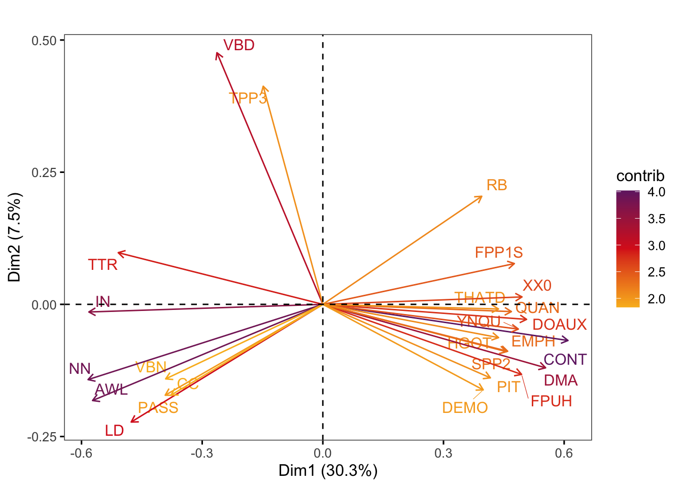

Code

#ggsave(here("plots", "fviz_pca_var_PC1_PC2_Ref3Reg.svg"), width = 9, height = 7)

factoextra::fviz_pca_var(pca,
             axes = c(3,2),
             select.var = list(contrib = 30),
             col.var = "contrib", # Colour by contributions to the PC
             gradient.cols = c("#F9B921", "#DB241E", "#722672"),
             title = "",
             repel = TRUE, # Try to avoid too much text overlapping
             ggtheme = ggthemes::theme_few())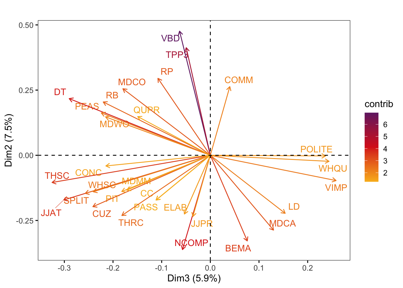

Code

#ggsave(here("plots", "fviz_pca_var_PC3_PC2_Ref3Reg.svg"), width = 9, height = 8)

factoextra::fviz_pca_var(pca,
             axes = c(3,4),
             select.var = list(contrib = 30),
             col.var = "contrib", # Colour by contributions to the PC
             gradient.cols = c("#F9B921", "#DB241E", "#722672"),
             title = "",
             repel = TRUE, # Try to avoid too much text overlapping
             ggtheme = ggthemes::theme_few())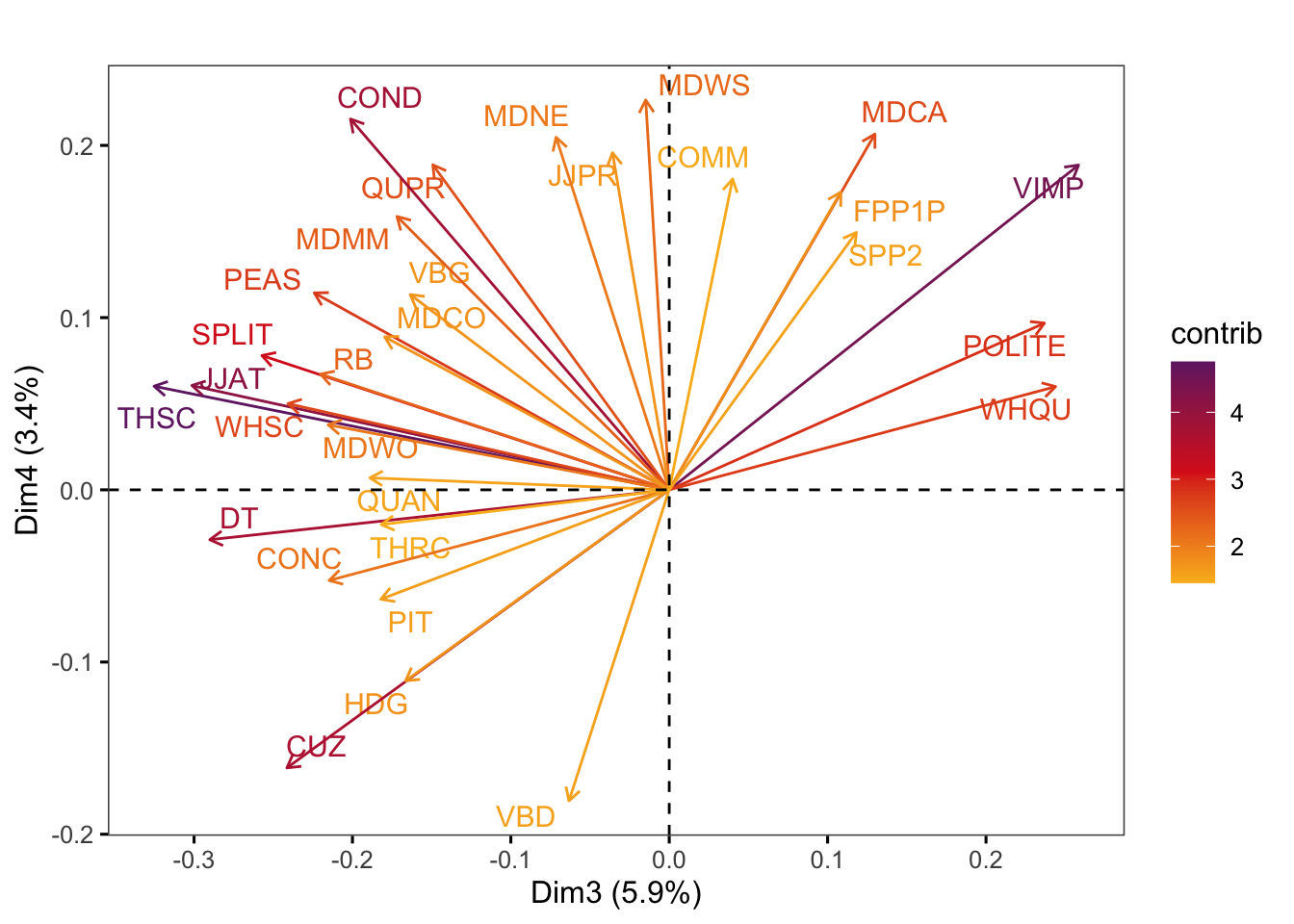

Code

#ggsave(here("plots", "fviz_pca_var_PC3_PC4_Ref3Reg.svg"), width = 9, height = 8)

H.7 Exploring feature contributions in terms of normalised frequencies

We can go back to the normalised frequencies of the individual features to compare them across different registers and levels, e.g.,:

Code

ncounts <- readRDS(here("data", "processed", "ncounts3_3Reg.rds"))

ncounts |> 
  filter(Register=="Informative") |> 
  #filter(Level %in% c("C", "D", "E")) |> 
  select(Level, VBD, PEAS) |> 
  group_by(Level) |> 
  summarise_if(is.numeric, mean) |> 
  kable(digits=2)

Level	VBD	PEAS
A	28.11	0.21
B	34.11	2.49
C	35.21	5.36
D	39.83	7.63
E	35.17	6.91
Ref.	39.73	4.94

The following chunk produces Figure 35 which shows normalised counts of selected features with salient loadings on PC1 in the Textbook Informative subcorpus (Levels A to E) and the reference Info Teens corpus (Ref.). This plots visualises the observed normalised frequencies as they were extracted using the MFTE Perl (see Appendices C and F).

Code

cols = c("#F9B921", "#A18A33", "#BD241E", "#722672", "#15274D", "darkgrey")

boxfeature <- ncounts |> 
  filter(Register=="Informative") |> 
  #filter(Level %in% c("C", "D", "E")) |> 
  select(Level, FPP1S, SPP2, CONT, EXIST, AWL, XX0, PASS, VBN) |> 
  ggplot(aes(x = Level, y = CONT, colour = Level, fill = Level)) +
  geom_jitter(size=0.7, alpha=.7) +
  geom_boxplot(outlier.shape = NA, fatten = 2, fill = "white", alpha = 0.3) +
  scale_colour_manual(values = cols) +
  theme_minimal() +
  theme(legend.position = "none") +
  xlab("")

CONT = boxfeature
SPP2 <- boxfeature + aes(y = SPP2) 
EXIST <- boxfeature + aes(y = EXIST) + ylim(c(0,25)) # These y-axis limits remove individual outliers that overextend the scales and make the existing differences invisible to the naked eye. They can be removed to visualise all data points.
FFP1 <- boxfeature + aes(y = FPP1S) + ylim(c(0,60))  
AWL <- boxfeature + aes(y = AWL)
XX0 <- boxfeature + aes(y = XX0) + ylim(c(0,25))
PASS <- boxfeature + aes(y = PASS)
VBN <- boxfeature + aes(y = VBN) + ylim(c(0,40))

boxplots <- gridExtra::grid.arrange(PASS, VBN, AWL, EXIST, FFP1, SPP2, CONT, XX0, ncol=2, nrow=4)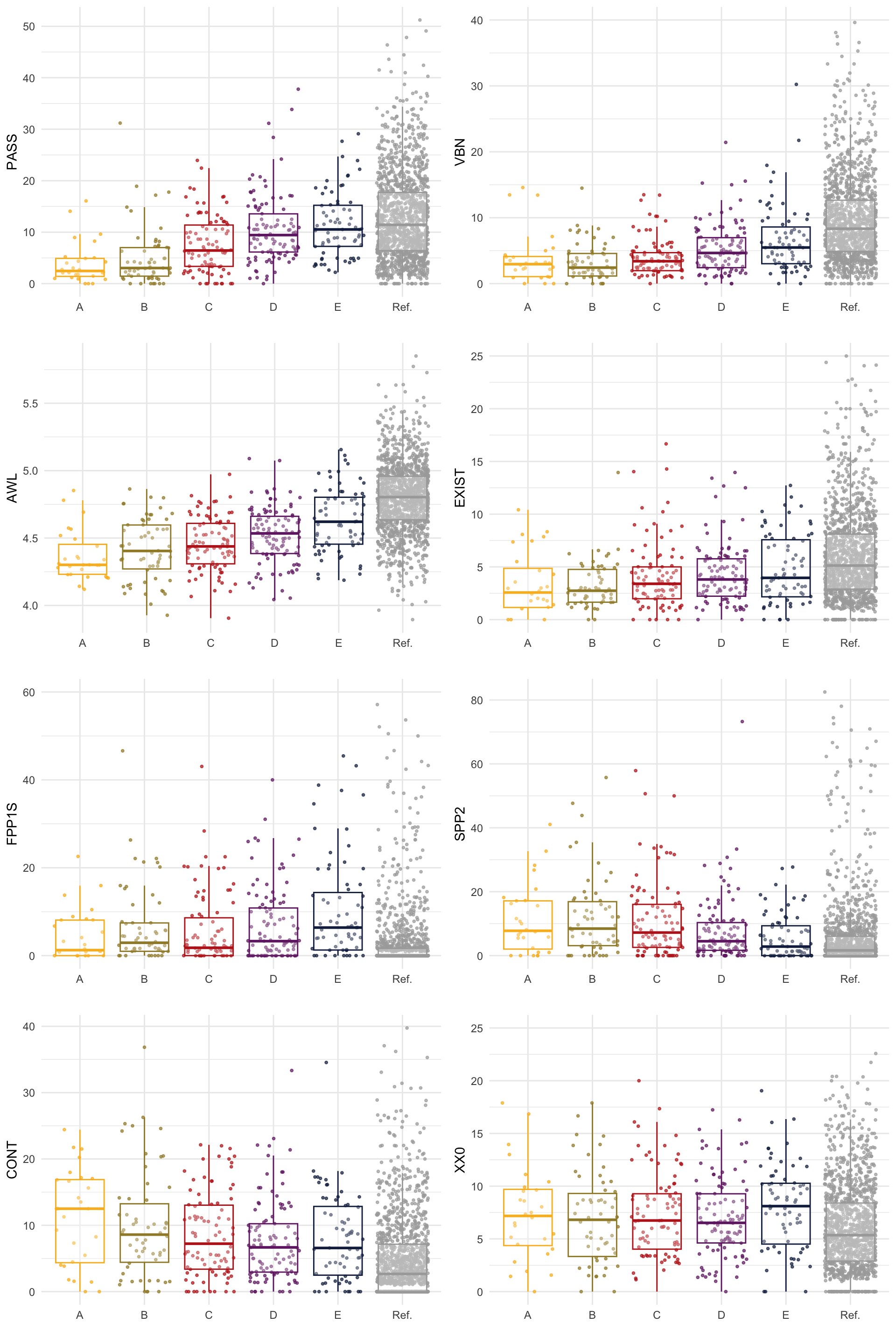

Code

#ggsave(here("plots", "BoxplotsInformativeFeatures.svg"), plot = boxplots, dpi = 300, width = 9, height = 11)

H.8 Exploring the dimensions of the model

We begin with some descriptive statistics of the dimension scores.

Code

#data <- readRDS(here("data", "processed", "dataforPCA.rds")) 
#colnames(data)
pca <- prcomp(data[,9:ncol(data)], scale.=FALSE) # All quantitative variables

## Access to the PCA results
#colnames(data)
res.ind <- cbind(data[,1:8], as.data.frame(pca$x)[,1:4])

## Summary statistics
res.ind |> 
  group_by(Subcorpus, Level) |> 
  summarise_if(is.numeric, c(mean = mean, sd = sd)) |> 
  kable(digits = 2)

Subcorpus	Level	Words_mean	PC1_mean	PC2_mean	PC3_mean	PC4_mean	Words_sd	PC1_sd	PC2_sd	PC3_sd	PC4_sd
Textbook Conversation	A	813.02	1.91	-1.02	3.49	-0.17	154.57	0.89	0.60	1.03	0.73
Textbook Conversation	B	819.48	2.11	-0.64	2.33	0.39	218.88	0.91	0.69	1.04	0.79
Textbook Conversation	C	823.69	1.59	-0.38	1.39	0.75	279.14	1.20	0.73	1.04	0.79
Textbook Conversation	D	797.85	1.09	-0.43	0.79	0.91	187.98	1.45	0.72	1.26	0.79
Textbook Conversation	E	1132.79	1.03	-0.61	0.86	1.09	569.85	1.30	0.78	0.88	0.62
Textbook Fiction	A	886.00	0.13	0.22	2.74	-0.27	242.78	0.97	0.69	0.90	0.81
Textbook Fiction	B	864.16	-0.21	1.34	1.73	-0.29	222.44	0.79	0.62	0.73	0.53
Textbook Fiction	C	854.21	-0.27	1.63	0.76	0.12	198.21	0.89	0.78	0.96	0.63
Textbook Fiction	D	801.78	-0.84	1.38	0.26	0.15	196.33	1.15	0.79	0.83	0.59
Textbook Fiction	E	853.26	-0.65	1.27	0.26	0.20	195.97	1.10	0.75	0.92	0.57
Textbook Informative	A	851.71	-1.46	-0.96	1.86	-0.70	199.77	0.82	0.86	0.69	0.85
Textbook Informative	B	844.03	-1.63	-0.50	1.23	-0.27	182.83	0.92	1.03	0.80	1.08
Textbook Informative	C	838.90	-1.87	-0.54	0.25	0.14	160.21	1.09	0.98	0.93	1.06
Textbook Informative	D	847.65	-2.24	-0.32	-0.15	0.13	179.25	0.95	0.92	0.95	0.83
Textbook Informative	E	823.23	-2.57	-0.66	-0.28	0.37	180.39	0.99	0.90	0.79	0.82
Spoken BNC2014 Ref.	Ref.	10637.74	3.71	-0.52	-0.64	-0.53	8974.14	0.49	0.47	0.76	0.52
Youth Fiction Ref.	Ref.	5944.78	-0.49	1.75	-0.21	0.41	198.64	0.90	0.52	0.88	0.52
Info Teens Ref.	Ref.	805.41	-3.06	-0.96	-0.23	-0.15	193.31	1.09	1.19	0.88	1.19

Code

res.ind <- res.ind |> 
  mutate(Subsubcorpus = paste(Corpus, Register, sep = "_")) |> 
  mutate(Subsubcorpus = as.factor(Subsubcorpus))
  
res.ind |> 
  select(PC1, PC2, PC3, PC4, Subsubcorpus) |> 
  tbl_summary(by = Subsubcorpus,
              digits = list(all_continuous() ~ c(2, 2)),
              statistic = all_continuous() ~  "{mean} ({sd})")

Characteristic	Informative.Teens_Informative, N = 1,337¹	Spoken.BNC2014_Conversation, N = 1,250¹	Textbook.English_Conversation, N = 565¹	Textbook.English_Fiction, N = 285¹	Textbook.English_Informative, N = 352¹	Youth.Fiction_Fiction, N = 1,191¹
PC1	-3.06 (1.09)	3.71 (0.49)	1.56 (1.25)	-0.43 (1.05)	-2.05 (1.04)	-0.49 (0.90)
PC2	-0.96 (1.19)	-0.52 (0.47)	-0.57 (0.74)	1.25 (0.84)	-0.52 (0.96)	1.75 (0.52)
PC3	-0.23 (0.88)	-0.64 (0.76)	1.71 (1.43)	0.96 (1.22)	0.31 (1.10)	-0.21 (0.88)
PC4	-0.15 (1.19)	-0.53 (0.52)	0.61 (0.86)	0.02 (0.64)	0.05 (0.98)	0.41 (0.52)
¹ Mean (SD)

Code

res.ind |> 
  select(Register, Level, PC4) |> 
  group_by(Register, Level) |> 
  summarise_if(is.numeric, c(Median = median, MAD = mad)) |> 
  kable(digits = 2)

Register	Level	Median	MAD
Conversation	A	-0.07	0.68
Conversation	B	0.42	0.80
Conversation	C	0.73	0.80
Conversation	D	0.86	0.70
Conversation	E	1.09	0.61
Conversation	Ref.	-0.54	0.52
Fiction	A	-0.38	0.75
Fiction	B	-0.39	0.53
Fiction	C	0.13	0.67
Fiction	D	0.01	0.54
Fiction	E	0.12	0.67
Fiction	Ref.	0.40	0.50
Informative	A	-0.71	0.82
Informative	B	-0.37	1.10
Informative	C	0.07	1.09
Informative	D	0.04	0.79
Informative	E	0.37	0.57
Informative	Ref.	-0.08	1.21

The following chunk can be used to search for example texts that are located in specific areas of the biplots. For example, we can search for texts that have high scores on Dim3 and low ones on Dim2 to proceed with a qualitative comparison and analysis of these texts.

Code

# Search for example texts to illustrate results
res.ind |> 
  filter(PC3 > 2 & PC2 < -2) |> 
  #filter(Register=="Conversation") |> 
  #filter(Level == "B") |> 
  #filter(PC1 > 4.7) |> 
  select(Filename, PC1, PC2, PC3) |> 
  kable(digits=2)

Filename	PC1	PC2	PC3
NGL_1_Spoken_0002.txt	2.41	-2.27	4.36
HT_5_ELF_Spoken_0003.txt	1.94	-2.30	3.49
HT_6_Informative_0001.txt	-2.19	-2.36	3.11
Science_Tech_Kinds_NZ_10383721_typesofrobots.txt	-3.09	-2.62	2.24
History_Kids_BBC_10402894_go_furthers.txt	-4.26	-2.07	2.08

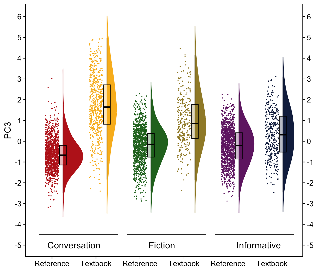
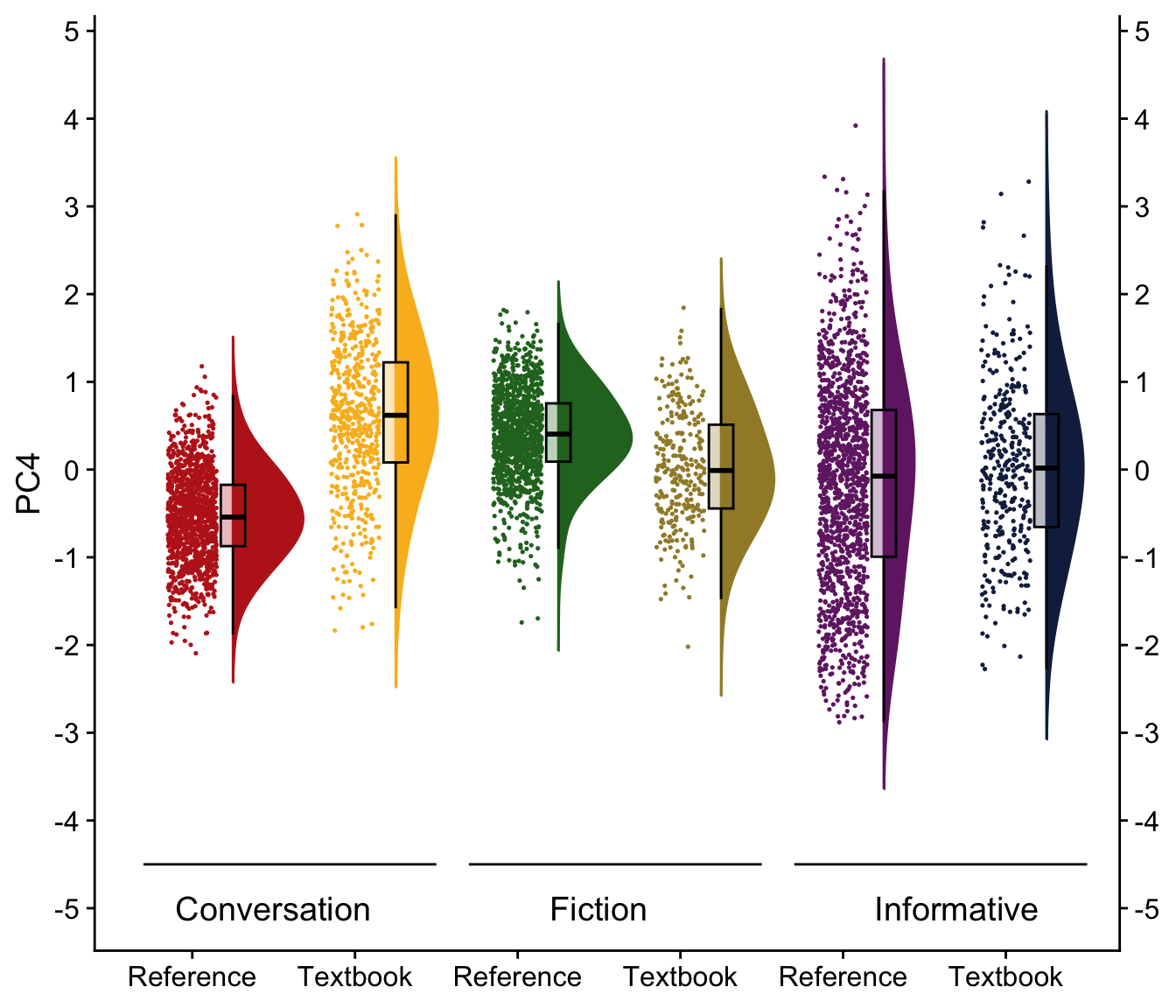
H.9 Raincloud plots visualising dimension scores

Code

res.ind$Subcorpus <- fct_relevel(res.ind$Subcorpus, "Spoken BNC2014 Ref.", "Textbook Conversation", "Youth Fiction Ref.", "Textbook Fiction", "Info Teens Ref.", "Textbook Informative")

# colours <- suf_palette(name = "london", n = 6, type = "continuous")
# colours2 <- suf_palette(name = "classic", n = 5, type = "continuous")
# colours <- c(colours, colours2[c(2:4)]) # Nine colours range
# palette <- colours[c(1,5,6,2,3,8,7,4,9)] # Good order for PCA
# colours <- palette[c(1,8,9,2,7,3)]

# This translates as:
palette <- c("#BD241E", "#A18A33", "#15274D", "#D54E1E", "#EA7E1E", "#4C4C4C", "#722672", "#F9B921", "#267226")
colours <- c("#BD241E", "#F9B921", "#267226", "#A18A33", "#722672","#15274D")

raincloud <- function(data, pc_var, from, to) {
  # Calculate the y-coordinates for the annotate() functions based on the bottom end of the y-axis ('from' argument)
  offset <- from + 7
  p <- ggplot(data, aes(x=Subcorpus, y=.data[[pc_var]], fill = Subcorpus, colour = Subcorpus))+
    geom_flat_violin(position = position_nudge(x = .25, y = 0),adjust = 2, trim = FALSE)+
    geom_point(position = position_jitter(width = .15), size = .25)+
    geom_boxplot(aes(x = as.numeric(Subcorpus)+0.25, y = .data[[pc_var]]), outlier.shape = NA, alpha = 0.3, width = .15, colour = "BLACK") +
    ylab(pc_var)+
    theme_cowplot()+
    theme(axis.title.x=element_blank())+
    guides(fill = "none", colour = "none") +
    scale_colour_manual(values = colours)+
    scale_fill_manual(values = colours) +
    annotate(geom = "text", x = 1.5, y = -7 + offset, label = "Conversation", size = 5) +
    annotate(geom = "segment", x = 0.7, xend = 2.5, y = -6.5 + offset, yend = -6.5 + offset) +
    annotate(geom = "text", x = 3.5, y = -7 + offset, label = "Fiction", size = 5) +
    annotate(geom = "segment", x = 2.7, xend = 4.5, y = -6.5 + offset, yend = -6.5 + offset) +
    annotate(geom = "text", x = 5.7, y = -7 + offset, label = "Informative", size = 5) +
    annotate(geom = "segment", x = 4.7, xend = 6.5, y = -6.5 + offset, yend = -6.5 + offset) +
    scale_x_discrete(labels=rep(c("Reference", "Textbook"), 3))+
    scale_y_continuous(sec.axis = dup_axis(name=NULL), breaks = seq(from = from, to = to, by = 1))
  return(p)
}

raincloud(res.ind, "PC1", -7, 5)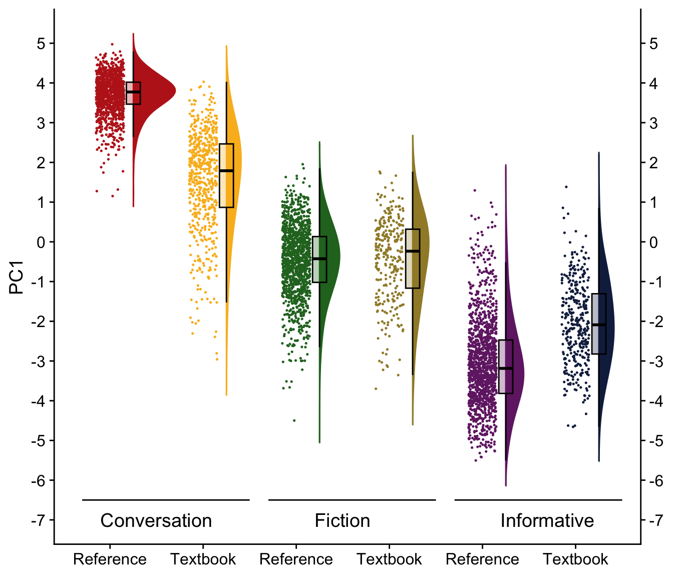

Code

#ggsave(here("plots", "PC1_3RegComparison.svg"), width = 13, height = 8)
#ggsave(here("plots", "PC1_3RegComparison.png"), width = 20, height = 15, units = "cm", dpi = 300)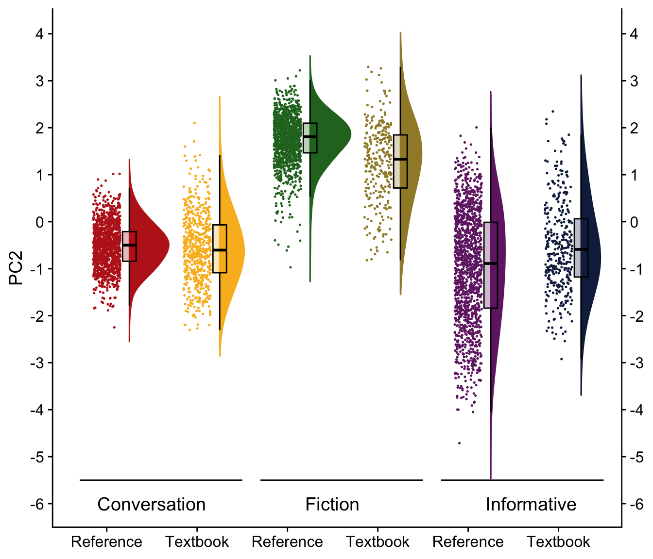

H.10 Computing mixed-effects models of the dimension scores

H.10.1 Data preparation

In this chunk, we add a Source variable to be used as a random effect variable in the following mixed-effects models (see 5.3.8 for details).

Code

res.ind <- res.ind |> 
  mutate(Source = case_when(
  Corpus=="Youth.Fiction" ~ paste("Book", str_extract(Filename, "[0-9]{1,3}"), sep = ""),
  Corpus=="Spoken.BNC2014" ~ "Spoken.BNC2014",
  Corpus=="Textbook.English" ~ as.character(Series),
  Corpus=="Informative.Teens" ~ str_extract(Filename, "BBC|Science_Tech"),
  TRUE ~ "NA")) |> 
  mutate(Source = case_when(
  Corpus=="Informative.Teens" & is.na(Source) ~ str_remove(Filename, "_.*"),
  TRUE ~ as.character(Source))) |> 
  mutate(Source = as.factor(Source)) |> 
  mutate(Corpus = case_when(
    Corpus=="Textbook.English" ~ "Textbook",
    Corpus=="Informative.Teens" ~ "Reference",
    Corpus=="Spoken.BNC2014" ~ "Reference",
    Corpus=="Youth.Fiction" ~ "Reference"
  )) |> 
  mutate(Corpus = as.factor(Corpus))

# Change the reference levels to theoretically more meaningful levels and one that is better populated (see, e.g., https://stats.stackexchange.com/questions/430770/in-a-multilevel-linear-regression-how-does-the-reference-level-affect-other-lev)
# summary(res.ind$Corpus)
res.ind$Corpus <- relevel(res.ind$Corpus, "Reference")

# summary(res.ind$Subcorpus)
res.ind$Subcorpus <- factor(res.ind$Subcorpus, levels = c("Spoken BNC2014 Ref.", "Textbook Conversation", "Youth Fiction Ref.", "Textbook Fiction", "Info Teens Ref.", "Textbook Informative"))

# summary(res.ind$Level)
res.ind$Level <- relevel(res.ind$Level, "Ref.")

H.10.2 Dimension 1: ‘Spontaneous interactional vs. Edited informational’

We first compare various models and then present a tabular summary of the best-fitting one.

md_source <- lmer(PC1 ~ 1 + (Register|Source), res.ind, REML = FALSE) 
md_corpus <- update(md_source, .~. + Level) # Failed to converge
md_register <- update(md_source, . ~ . + Register)
md_both <- update(md_corpus, .~. + Register)
md_interaction <- update(md_both, . ~ . + Level:Register)

anova(md_source, md_corpus, md_register, md_both, md_interaction)

Data: res.ind
Models:
md_source: PC1 ~ 1 + (Register | Source)
md_register: PC1 ~ (Register | Source) + Register
md_corpus: PC1 ~ (Register | Source) + Level
md_both: PC1 ~ (Register | Source) + Level + Register
md_interaction: PC1 ~ (Register | Source) + Level + Register + Level:Register
               npar   AIC   BIC  logLik deviance   Chisq Df Pr(>Chisq)    
md_source         8 12421 12473 -6202.5    12405                          
md_register      10 12357 12422 -6168.4    12337  68.106  2  1.625e-15 ***
md_corpus        13 12181 12266 -6077.5    12155 181.996  3  < 2.2e-16 ***
md_both          15 12117 12215 -6043.5    12087  67.843  2  1.854e-15 ***
md_interaction   25 12098 12261 -6024.0    12048  39.104 10  2.435e-05 ***
---
Signif. codes:  0 '***' 0.001 '**' 0.01 '*' 0.05 '.' 0.1 ' ' 1

md_interaction <- lmer(PC1 ~ Level + Register + Level*Register + (Register|Source), res.ind, REML = FALSE) 

tab_model(md_interaction, wrap.labels = 200) # R2 = 0.870 / 0.923

	PC 1
Predictors	Estimates	CI	p
(Intercept)	3.71	2.46 – 4.96	<0.001
Level [A]	-1.73	-3.06 – -0.40	0.011
Level [B]	-1.65	-2.97 – -0.32	0.015
Level [C]	-2.08	-3.40 – -0.76	0.002
Level [D]	-2.47	-3.80 – -1.15	<0.001
Level [E]	-2.73	-4.06 – -1.40	<0.001
Register [Fiction]	-4.20	-5.45 – -2.95	<0.001
Register [Informative]	-6.75	-8.03 – -5.47	<0.001
Level [A] × Register [Fiction]	2.18	0.86 – 3.49	0.001
Level [B] × Register [Fiction]	1.71	0.41 – 3.01	0.010
Level [C] × Register [Fiction]	2.12	0.83 – 3.42	0.001
Level [D] × Register [Fiction]	1.93	0.64 – 3.23	0.003
Level [E] × Register [Fiction]	2.41	1.10 – 3.71	<0.001
Level [A] × Register [Informative]	3.37	2.01 – 4.73	<0.001
Level [B] × Register [Informative]	3.17	1.83 – 4.51	<0.001
Level [C] × Register [Informative]	3.24	1.90 – 4.57	<0.001
Level [D] × Register [Informative]	3.20	1.87 – 4.53	<0.001
Level [E] × Register [Informative]	3.14	1.80 – 4.48	<0.001
Random Effects
σ²	0.59
τ₀₀_Source	0.41
τ₁₁_{Source.RegisterFiction}	0.12
τ₁₁_{Source.RegisterInformative}	0.20
ρ₀₁	-0.05
	-0.48
ICC	0.41
N _Source	325
Observations	4980
Marginal R² / Conditional R²	0.870 / 0.923

Its estimated coefficients are visualised in the plot below.

Code

# Tweak plot aesthetics with: https://cran.r-project.org/web/packages/sjPlot/vignettes/custplot.html
# Colour customisation trick from: https://stackoverflow.com/questions/55598920/different-line-colors-in-forest-plot-output-from-sjplot-r-package

plot_model(md_interaction, 
           #type = "re", # Option to visualise random effects 
           show.intercept = TRUE,
           show.values=TRUE, 
           show.p=TRUE,
           value.offset = .4,
           value.size = 3.5,
           colors = palette[c(1:3,7:9)],
           group.terms = c(1,5,5,5,5,5,6,4,2,2,2,2,2,3,3,3,3,3), 
           title="Fixed effects",
           wrap.labels = 40,
           axis.title = "PC1 estimated coefficients") +
  theme_sjplot2()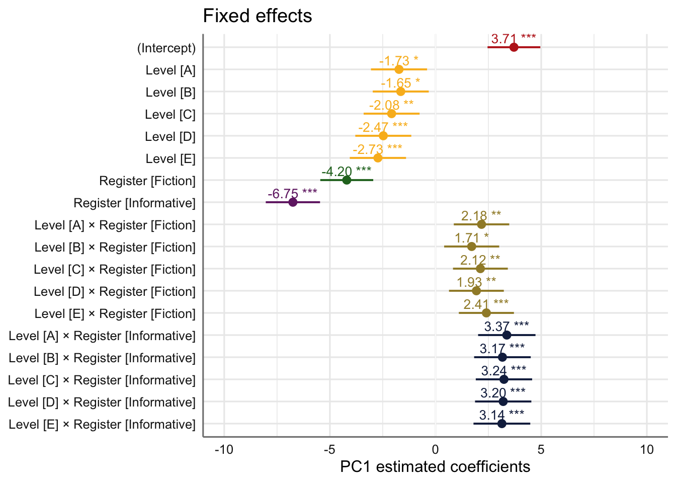

Code

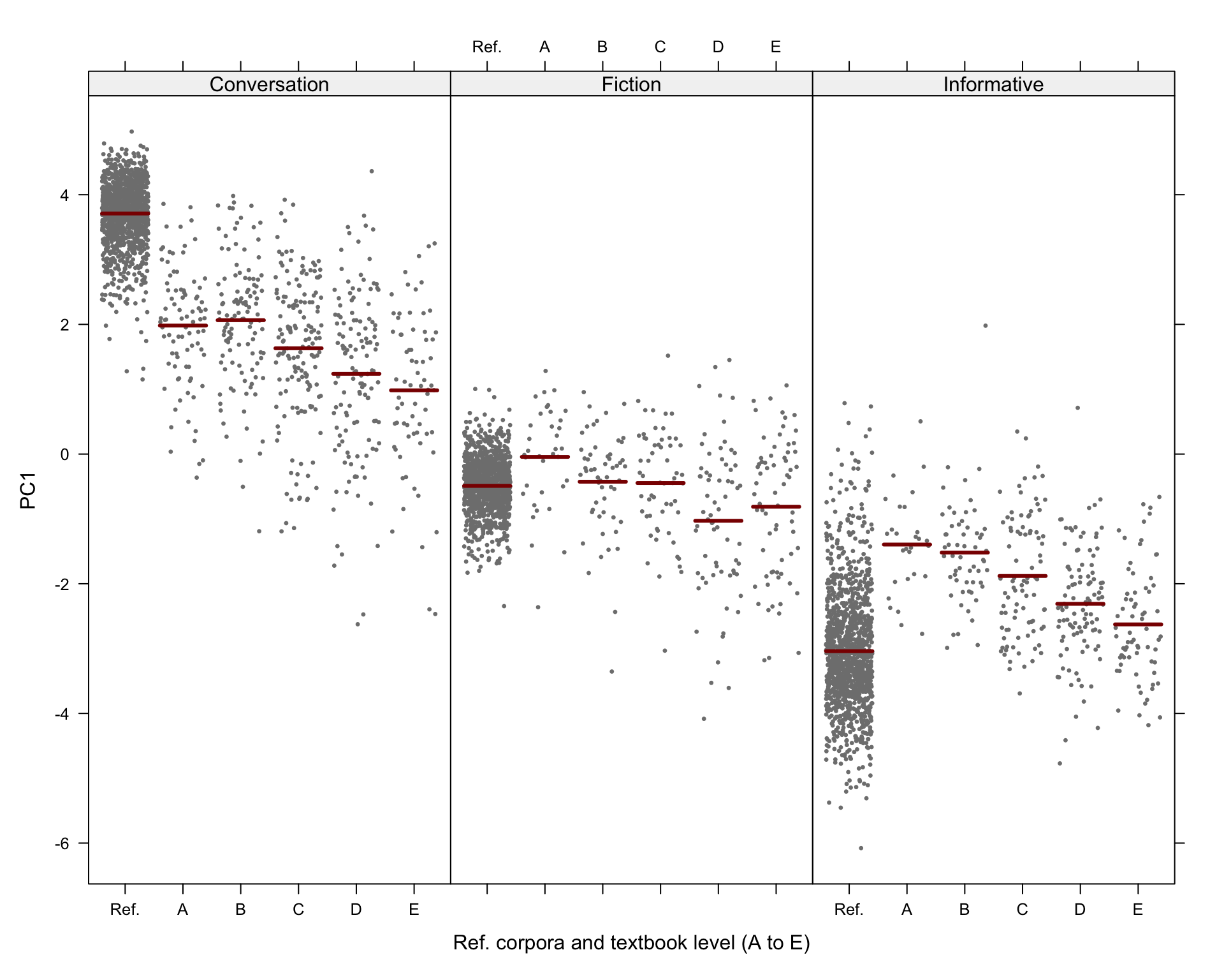
#ggsave(here("plots", "TxBRef3Reg_PC1_lmer_fixed.svg"), height = 6, width = 9)

The visreg function is used to visualise the distributions of the modelled Dim1 scores:

Code

# svg(here("plots", "TxBReg3Reg_predicted_PC1_scores_interactions.svg"), height = 8, width = 9)
visreg(md_interaction, xvar = "Level", by="Register", 
       #type = "contrast",
       type = "conditional",
       line=list(col="darkred"), 
       points=list(cex=0.3),
       xlab = "Ref. corpora and textbook level (A to E)", ylab = "PC1",
       layout=c(3,1)
)

Code

# dev.off()

For PC2 to PC4, the models with random intercepts and slopes failed to converge, which is why only slopes are included in the following models.

Code

# Function to avoid repeating model fitting and comparison process for each PC.
run_anova <- function(response_var, data) {
  # Fit the initial model
  md_source <- lmer(formula = paste(response_var, "~ 1 + (1|Source)"), data = data, REML = FALSE)
  
  # Update models
  md_corpus <- update(md_source, . ~ . + Level)
  md_register <- update(md_source, . ~ . + Register)
  md_both <- update(md_corpus, . ~ . + Register)
  md_interaction <- update(md_both, . ~ . + Level:Register)
  
  # Perform ANOVA
  anova_results <- anova(md_source, md_corpus, md_register, md_both, md_interaction)
  
  # Print ANOVA results
  print(anova_results)
  
  # Save model object with appropriate name
  pc_number <- gsub("PC", "", response_var)
  assign(paste("md_interaction_PC", pc_number, sep = ""), md_interaction, envir = .GlobalEnv)
  
  # Return tabulated model
  return(md_interaction)
}

H.10.3 Dimension 2: ‘Narrative vs. Non-narrative’

We first compare various models and then present a tabular summary of the best-fitting one.

PC2_models <- run_anova("PC2", res.ind)

Data: data
Models:
md_source: PC2 ~ 1 + (1 | Source)
md_register: PC2 ~ (1 | Source) + Register
md_corpus: PC2 ~ (1 | Source) + Level
md_both: PC2 ~ (1 | Source) + Level + Register
md_interaction: PC2 ~ (1 | Source) + Level + Register + Level:Register
               npar   AIC   BIC  logLik deviance    Chisq Df Pr(>Chisq)    
md_source         3 12281 12301 -6137.6    12275                           
md_register       5 10761 10794 -5375.7    10751 1523.882  2  < 2.2e-16 ***
md_corpus         8 12138 12190 -6061.1    12122    0.000  3          1    
md_both          10 10616 10681 -5298.1    10596 1525.963  2  < 2.2e-16 ***
md_interaction   20 10550 10680 -5254.9    10510   86.436 10  2.718e-14 ***
---
Signif. codes:  0 '***' 0.001 '**' 0.01 '*' 0.05 '.' 0.1 ' ' 1

tab_model(md_interaction_PC2) # R2 = 0.671 / 0.753

	PC 2
Predictors	Estimates	CI	p
(Intercept)	-0.52	-1.27 – 0.24	0.183
Level [A]	-0.54	-1.35 – 0.28	0.195
Level [B]	-0.15	-0.96 – 0.66	0.721
Level [C]	0.08	-0.72 – 0.89	0.842
Level [D]	0.04	-0.76 – 0.85	0.915
Level [E]	0.07	-0.75 – 0.89	0.866
Register [Fiction]	2.27	1.51 – 3.03	<0.001
Register [Informative]	-0.46	-1.24 – 0.32	0.250
Level [A] × Register [Fiction]	-1.01	-1.82 – -0.21	0.014
Level [B] × Register [Fiction]	-0.25	-1.04 – 0.54	0.532
Level [C] × Register [Fiction]	-0.21	-1.00 – 0.58	0.602
Level [D] × Register [Fiction]	-0.41	-1.20 – 0.38	0.308
Level [E] × Register [Fiction]	-0.47	-1.26 – 0.32	0.246
Level [A] × Register [Informative]	0.49	-0.34 – 1.33	0.246
Level [B] × Register [Informative]	0.59	-0.22 – 1.40	0.154
Level [C] × Register [Informative]	0.26	-0.54 – 1.06	0.524
Level [D] × Register [Informative]	0.55	-0.26 – 1.35	0.183
Level [E] × Register [Informative]	0.33	-0.49 – 1.14	0.431
Random Effects
σ²	0.45
τ₀₀_Source	0.15
ICC	0.25
N _Source	325
Observations	4980
Marginal R² / Conditional R²	0.671 / 0.753

Visualisation of the coefficient estimates of the fixed effects:

Code

plot_model(md_interaction_PC2, 
           #type = "re", # Option to visualise random effects 
           show.intercept = TRUE,
           show.values=TRUE, 
           show.p=TRUE,
           value.offset = .4,
           value.size = 3.5,
           colors = palette[c(1:3,7:9)],
           group.terms = c(1,5,5,5,5,5,6,4,2,2,2,2,2,3,3,3,3,3), 
           title="Fixed effects",
           wrap.labels = 40,
           axis.title = "PC2 estimated coefficients") +
  theme_sjplot2()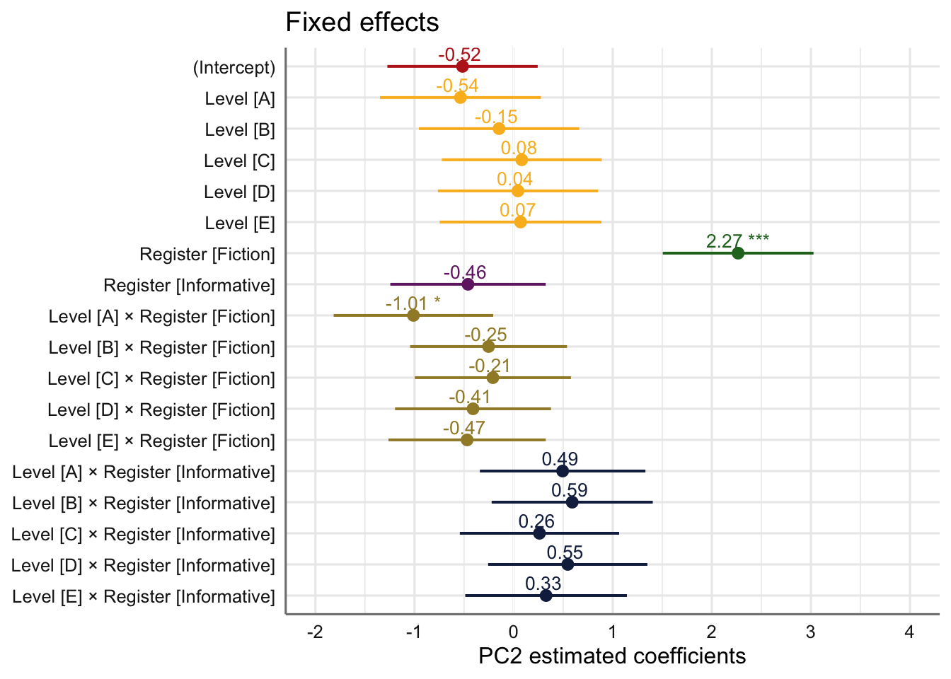

Code

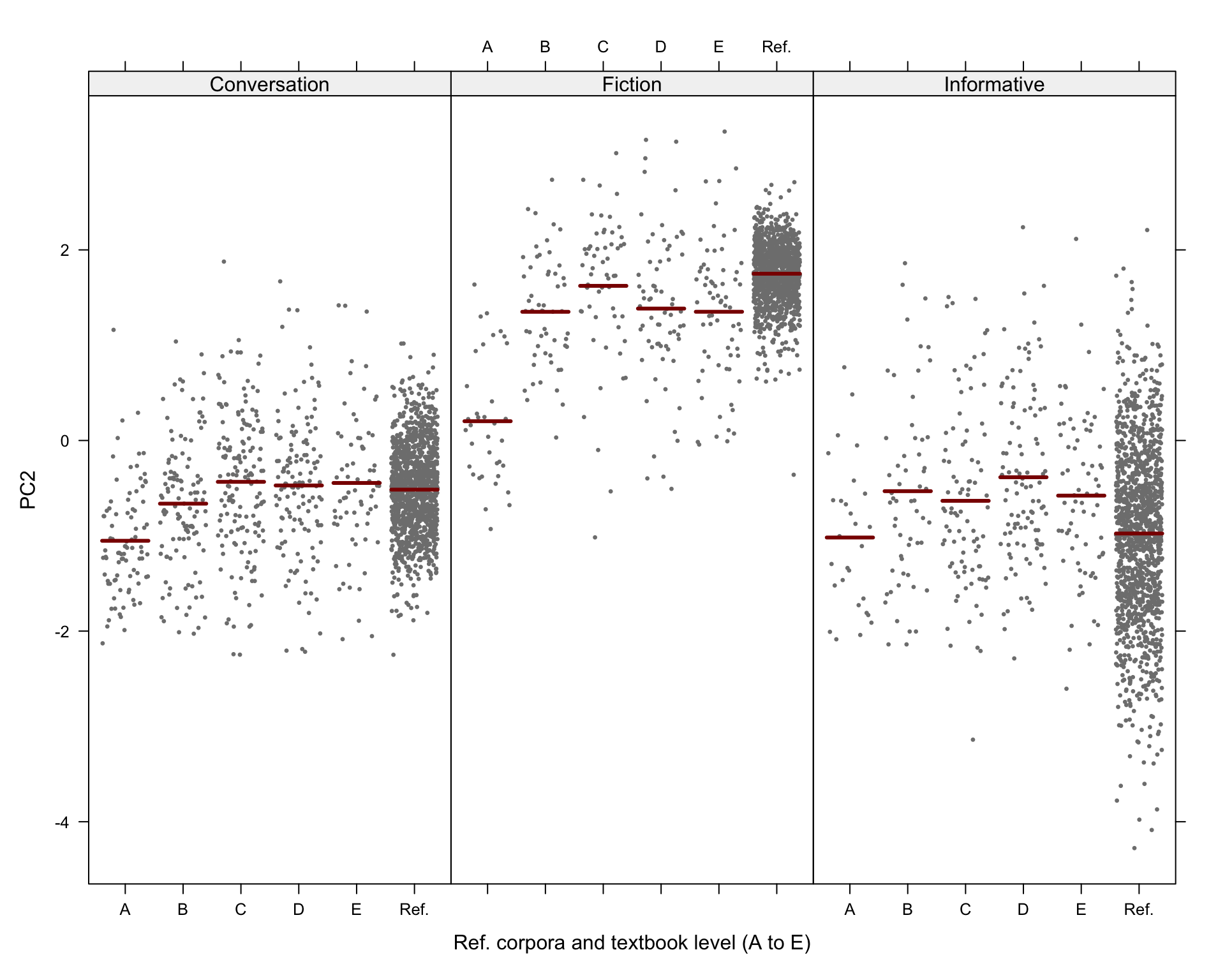
#ggsave(here("plots", "TxBRef3Reg_PC2_lmer_fixed.svg"), height = 6, width = 9)

Visualisation of the predicted Dim2 scores:

Code

# svg(here("plots", "TxBReg3Reg_predicted_PC2_scores_interactions.svg"), height = 8, width = 9)
visreg(md_interaction_PC2, xvar = "Level", by="Register", 
       #type = "contrast",
       type = "conditional",
       line=list(col="darkred"), 
       points=list(cex=0.3),
       xlab = "Ref. corpora and textbook level (A to E)", ylab = "PC2",
       layout=c(3,1)
)

Code

# dev.off()

We can also explore the random effect structure.

# Random effects
ranef <- as.data.frame(ranef(md_interaction_PC2))

# Exploring the random effects of the sources of the Info Teens corpus
ranef |> 
  filter(grp %in% c("TeenVogue", "BBC", "Dogo", "Ducksters", "Encyclopedia", "Factmonster", "History", "Quatr", "Revision", "Science", "Science_Tech", "Teen", "TweenTribute", "WhyFiles", "World")) |> 
  ggplot(aes(x = grp, y = condval)) +
  geom_point() +
  coord_flip()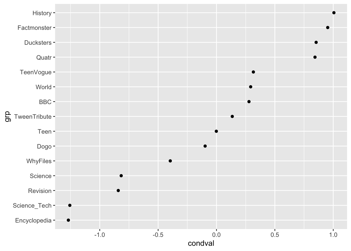

# Exploring the random effects associated with textbook series
ranef |> 
  filter(grp %in% levels(data$Series)) |> 
  ggplot(aes(x = grp, y = condval)) +
  geom_point() +
  coord_flip()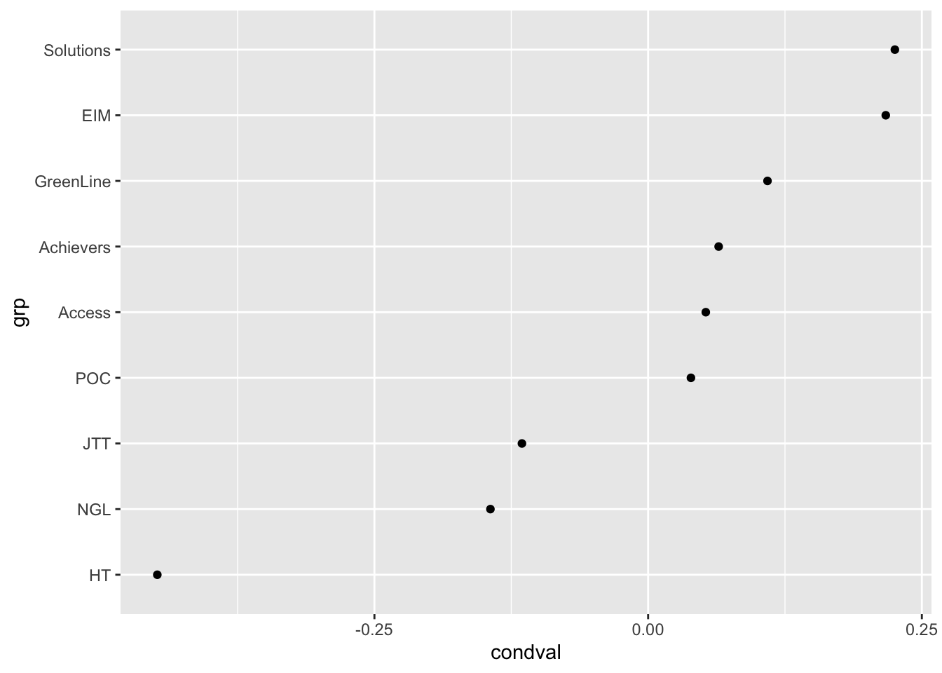

H.10.4 Dimension 3: ‘Pedagogically adapted vs. Natural’

We first compare various models and then present a tabular summary of the best-fitting one.

PC3_models <- run_anova("PC3", res.ind)

Data: data
Models:
md_source: PC3 ~ 1 + (1 | Source)
md_register: PC3 ~ (1 | Source) + Register
md_corpus: PC3 ~ (1 | Source) + Level
md_both: PC3 ~ (1 | Source) + Level + Register
md_interaction: PC3 ~ (1 | Source) + Level + Register + Level:Register
               npar   AIC   BIC  logLik deviance    Chisq Df Pr(>Chisq)    
md_source         3 13523 13542 -6758.3    13517                           
md_register       5 12988 13020 -6489.0    12978  538.750  2  < 2.2e-16 ***
md_corpus         8 11928 11981 -5956.2    11912 1065.455  3  < 2.2e-16 ***
md_both          10 11466 11531 -5722.8    11446  466.870  2  < 2.2e-16 ***
md_interaction   20 11461 11592 -5710.7    11421   24.264 10   0.006929 ** 
---
Signif. codes:  0 '***' 0.001 '**' 0.01 '*' 0.05 '.' 0.1 ' ' 1

tab_model(md_interaction_PC3) # R2 = 0.425 / 0.700

	PC 3
Predictors	Estimates	CI	p
(Intercept)	-0.64	-1.99 – 0.71	0.354
Level [A]	4.25	2.82 – 5.69	<0.001
Level [B]	3.09	1.66 – 4.52	<0.001
Level [C]	2.12	0.69 – 3.55	0.004
Level [D]	1.64	0.21 – 3.07	0.024
Level [E]	1.29	-0.15 – 2.73	0.078
Register [Fiction]	0.43	-0.92 – 1.79	0.533
Register [Informative]	0.43	-0.96 – 1.83	0.544
Level [A] × Register [Fiction]	-1.50	-2.89 – -0.12	0.033
Level [B] × Register [Fiction]	-1.39	-2.76 – -0.01	0.048
Level [C] × Register [Fiction]	-1.34	-2.71 – 0.03	0.056
Level [D] × Register [Fiction]	-1.35	-2.72 – 0.03	0.055
Level [E] × Register [Fiction]	-1.03	-2.41 – 0.35	0.142
Level [A] × Register [Informative]	-1.92	-3.35 – -0.49	0.009
Level [B] × Register [Informative]	-1.45	-2.86 – -0.03	0.045
Level [C] × Register [Informative]	-1.36	-2.77 – 0.05	0.058
Level [D] × Register [Informative]	-1.43	-2.84 – -0.02	0.047
Level [E] × Register [Informative]	-1.53	-2.95 – -0.11	0.034
Random Effects
σ²	0.52
τ₀₀_Source	0.48
ICC	0.48
N _Source	325
Observations	4980
Marginal R² / Conditional R²	0.425 / 0.700

Visualisation of the coefficient estimates of the fixed effects:

Code

plot_model(md_interaction_PC3, 
           #type = "re", # Option to visualise random effects 
           show.intercept = TRUE,
           show.values=TRUE, 
           show.p=TRUE,
           value.offset = .4,
           value.size = 3.5,
           colors = palette[c(1:3,7:9)],
           group.terms = c(1,5,5,5,5,5,6,4,2,2,2,2,2,3,3,3,3,3), 
           title="Fixed effects",
           wrap.labels = 40,
           axis.title = "PC3 estimated coefficients") +
  theme_sjplot2()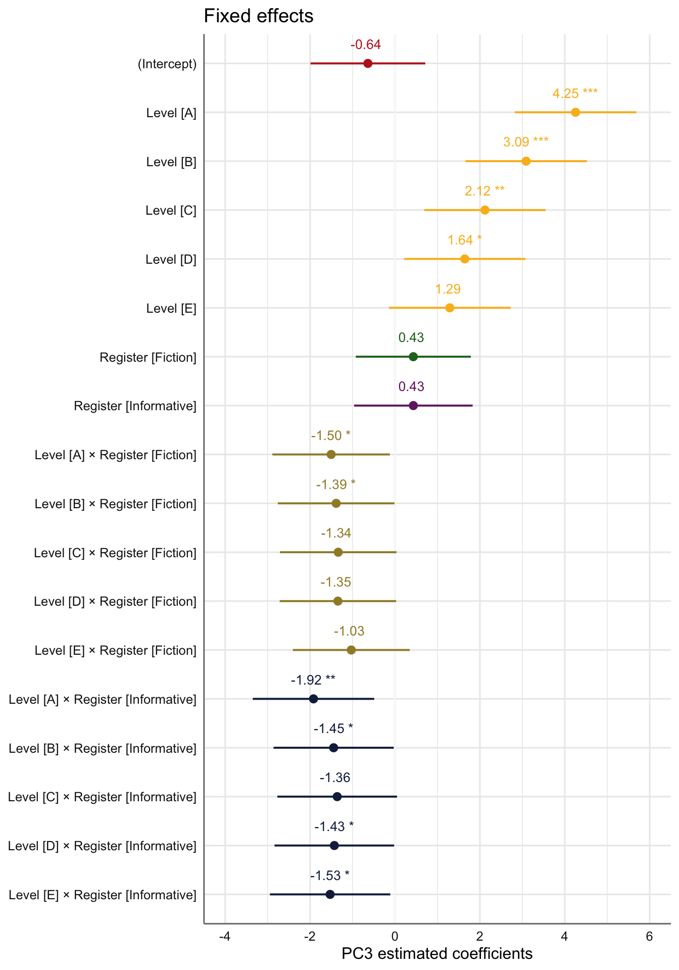

Code

#ggsave(here("plots", "TxBRef3Reg_PC3_lmer_fixed.svg"), height = 6, width = 9)

Visualisation of the predicted Dim3 scores:

Code

# svg(here("plots", "TxBReg3Reg_predicted_PC3_scores_interactions.svg"), height = 8, width = 9)
visreg(md_interaction_PC3, xvar = "Level", by="Register", 
       #type = "contrast",
       type = "conditional",
       line=list(col="darkred"), 
       points=list(cex=0.3),
       xlab = "Ref. corpora and textbook level (A to E)", ylab = "PC3",
       layout=c(3,1)
)

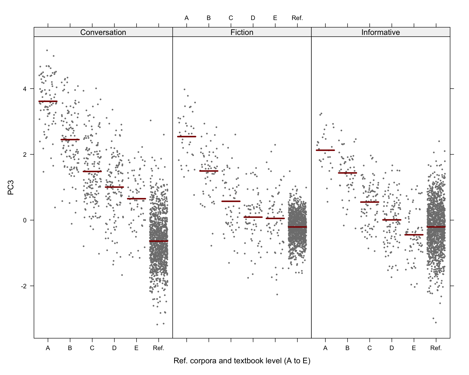
Code

# dev.off()

We can also explore the random effect structure.

# Random effects
ranef <- as.data.frame(ranef(md_interaction_PC3))

# Exploring the random effects of the sources of the Info Teens corpus
ranef |> 
  filter(grp %in% c("TeenVogue", "BBC", "Dogo", "Ducksters", "Encyclopedia", "Factmonster", "History", "Quatr", "Revision", "Science", "Science_Tech", "Teen", "TweenTribute", "WhyFiles", "World")) |> 
  ggplot(aes(x = grp, y = condval)) +
  geom_point() +
  coord_flip()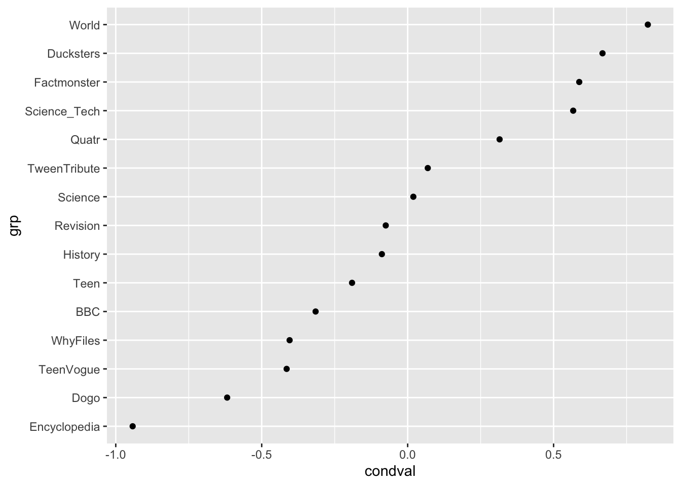

# Exploring the random effects associated with textbook series
ranef |> 
  filter(grp %in% levels(data$Series)) |> 
  ggplot(aes(x = grp, y = condval)) +
  geom_point() +
  coord_flip()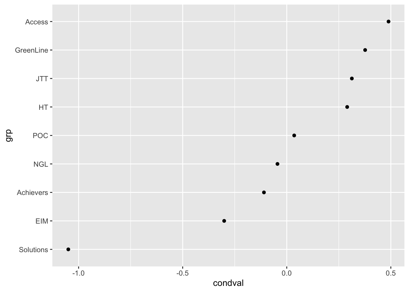

H.10.5 Dimension 4: ‘Factual vs. Speculative’ / ‘Simple vs. complex verb forms’?

We first compare various models and then present a tabular summary of the best-fitting one.

PC4_models <- run_anova("PC4", res.ind)

Data: data
Models:
md_source: PC4 ~ 1 + (1 | Source)
md_register: PC4 ~ (1 | Source) + Register
md_corpus: PC4 ~ (1 | Source) + Level
md_both: PC4 ~ (1 | Source) + Level + Register
md_interaction: PC4 ~ (1 | Source) + Level + Register + Level:Register
               npar   AIC   BIC  logLik deviance    Chisq Df Pr(>Chisq)    
md_source         3 11019 11039 -5506.5    11013                           
md_register       5 10825 10857 -5407.4    10815 198.2593  2    < 2e-16 ***
md_corpus         8 10827 10879 -5405.3    10811   4.0956  3     0.2513    
md_both          10 10563 10628 -5271.6    10543 267.5805  2    < 2e-16 ***
md_interaction   20 10527 10657 -5243.3    10487  56.4370 10    1.7e-08 ***
---
Signif. codes:  0 '***' 0.001 '**' 0.01 '*' 0.05 '.' 0.1 ' ' 1

tab_model(md_interaction_PC4) # R2 = 0.234 / 0.434

	PC 4
Predictors	Estimates	CI	p
(Intercept)	-0.53	-1.31 – 0.25	0.187
Level [A]	0.36	-0.47 – 1.20	0.392
Level [B]	0.91	0.08 – 1.74	0.033
Level [C]	1.28	0.45 – 2.11	0.003
Level [D]	1.45	0.62 – 2.28	0.001
Level [E]	1.64	0.80 – 2.47	<0.001
Register [Fiction]	0.93	0.15 – 1.71	0.019
Register [Informative]	0.38	-0.43 – 1.18	0.358
Level [A] × Register [Fiction]	-1.11	-1.94 – -0.29	0.008
Level [B] × Register [Fiction]	-1.67	-2.48 – -0.85	<0.001
Level [C] × Register [Fiction]	-1.59	-2.40 – -0.78	<0.001
Level [D] × Register [Fiction]	-1.75	-2.55 – -0.94	<0.001
Level [E] × Register [Fiction]	-1.86	-2.67 – -1.05	<0.001
Level [A] × Register [Informative]	-0.92	-1.78 – -0.07	0.034
Level [B] × Register [Informative]	-1.02	-1.85 – -0.19	0.016
Level [C] × Register [Informative]	-1.00	-1.83 – -0.18	0.017
Level [D] × Register [Informative]	-1.20	-2.03 – -0.38	0.004
Level [E] × Register [Informative]	-1.16	-1.99 – -0.32	0.007
Random Effects
σ²	0.45
τ₀₀_Source	0.16
ICC	0.26
N _Source	325
Observations	4980
Marginal R² / Conditional R²	0.234 / 0.434

Visualisation of the coefficient estimates of the fixed effects:

Code

plot_model(md_interaction_PC4, 
           #type = "re", # Option to visualise random effects 
           show.intercept = TRUE,
           show.values=TRUE, 
           show.p=TRUE,
           value.offset = .4,
           value.size = 3.5,
           colors = palette[c(1:3,7:9)],
           group.terms = c(1,5,5,5,5,5,6,4,2,2,2,2,2,3,3,3,3,3), 
           title="Fixed effects",
           wrap.labels = 40,
           axis.title = "PC4 estimated coefficients") +
  theme_sjplot2()

Code

#ggsave(here("plots", "TxBRef3Reg_PC4_lmer_fixed.svg"), height = 6, width = 9)

Visualisation of the predicted Dim4 scores:

Code

# svg(here("plots", "TxBReg3Reg_predicted_PC4_scores_interactions.svg"), height = 8, width = 9)
visreg(md_interaction_PC4, xvar = "Level", by="Register", 
       #type = "contrast",
       type = "conditional",
       line=list(col="darkred"), 
       points=list(cex=0.3),
       xlab = "Ref. corpora and textbook level (A to E)", ylab = "PC4",
       layout=c(3,1)
)

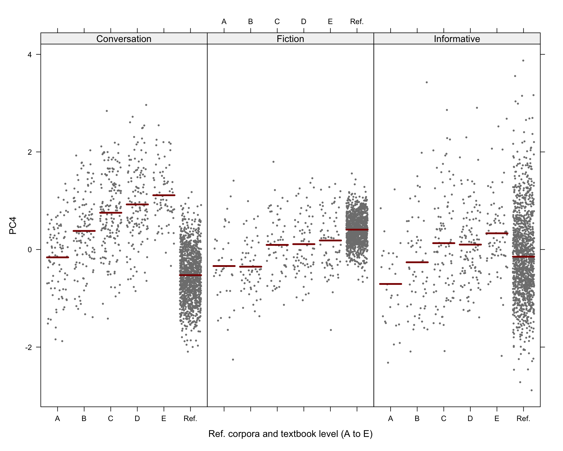
Code

# dev.off()

We can also explore the random effect structure.

# Random effects
ranef <- as.data.frame(ranef(md_interaction_PC4))

# Exploring the random effects of the sources of the Info Teens corpus
ranef |> 
  filter(grp %in% c("TeenVogue", "BBC", "Dogo", "Ducksters", "Encyclopedia", "Factmonster", "History", "Quatr", "Revision", "Science", "Science_Tech", "Teen", "TweenTribute", "WhyFiles", "World")) |> 
  ggplot(aes(x = grp, y = condval)) +
  geom_point() +
  coord_flip()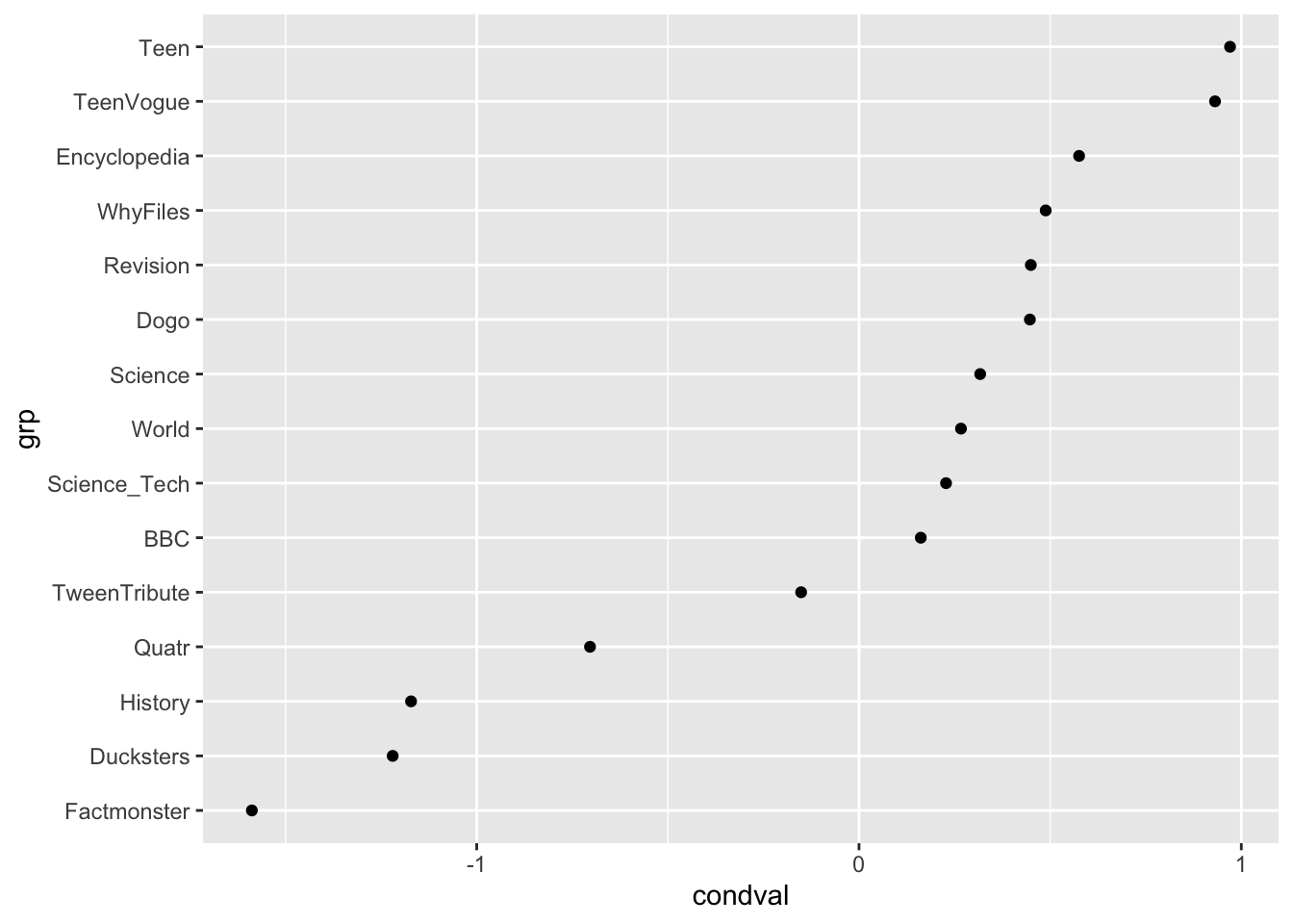

# Exploring the random effects associated with textbook series
ranef |> 
  filter(grp %in% levels(data$Series)) |> 
  ggplot(aes(x = grp, y = condval)) +
  geom_point() +
  coord_flip()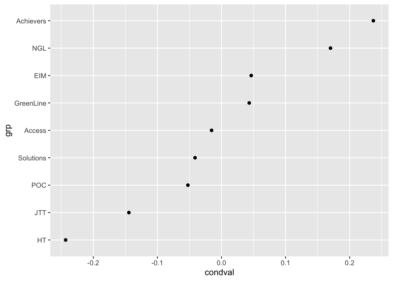

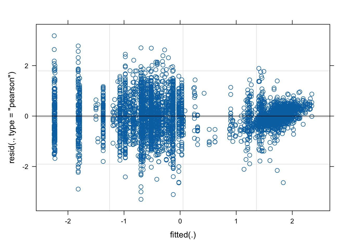
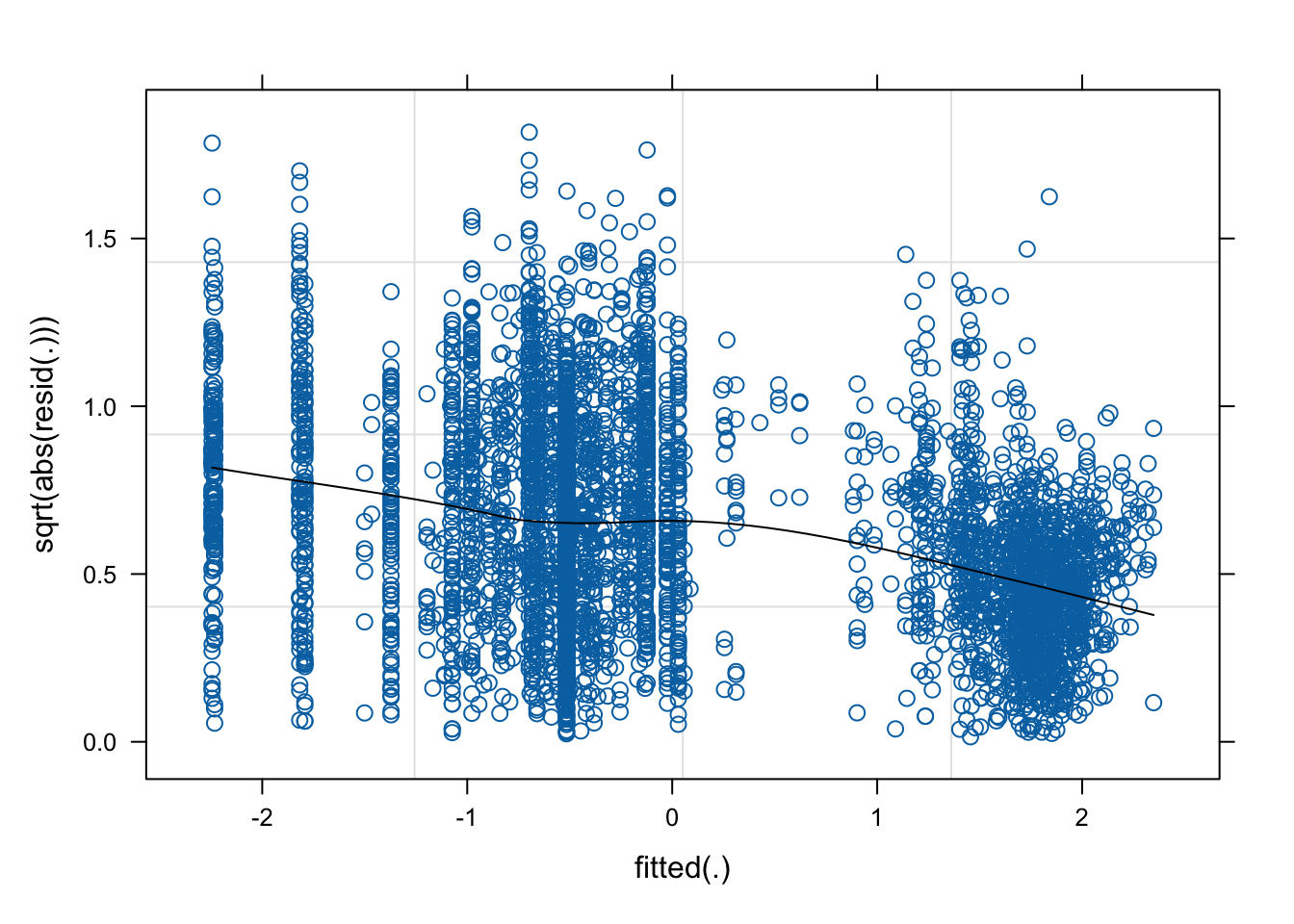
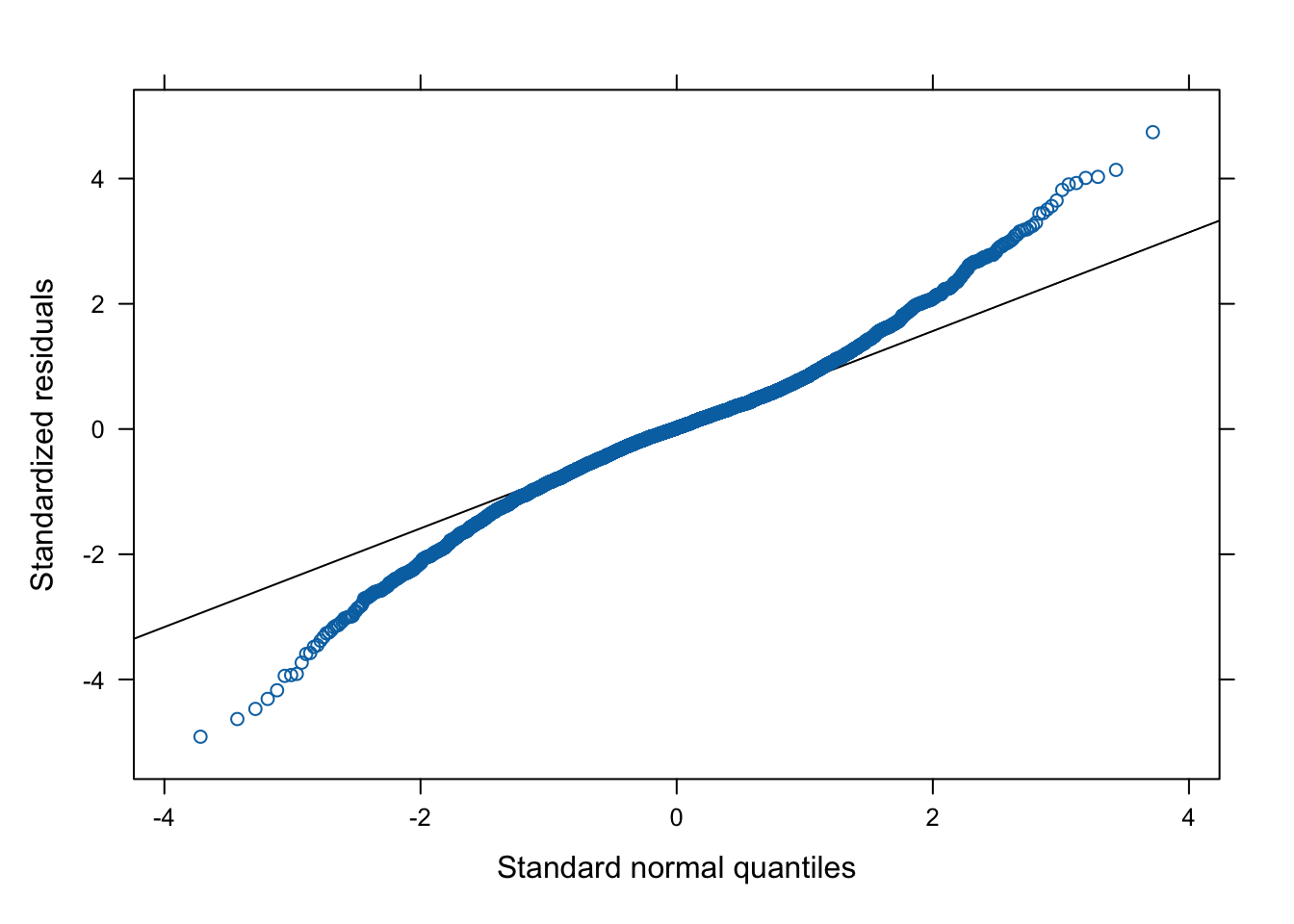
H.10.6 Testing model assumptions

This chunk can be used to check the assumptions of all of the models computed above. In the following example, we examine the final model selected to predict Dim2 scores.

model2test <- md_interaction_PC2

# check distribution of residuals
plot(model2test)

# scale-location plot
plot(model2test,
     sqrt(abs(resid(.)))~fitted(.),
     type=c("p","smooth"), col.line=1)

# Q-Q plot
lattice::qqmath(model2test)

H.11 Packages used in this script

H.11.1 Package names and versions

R version 4.4.1 (2024-06-14)
Platform: aarch64-apple-darwin20
Running under: macOS Sonoma 14.5

Matrix products: default
BLAS:   /Library/Frameworks/R.framework/Versions/4.4-arm64/Resources/lib/libRblas.0.dylib 
LAPACK: /Library/Frameworks/R.framework/Versions/4.4-arm64/Resources/lib/libRlapack.dylib;  LAPACK version 3.12.0

locale:
[1] en_US.UTF-8/en_US.UTF-8/en_US.UTF-8/C/en_US.UTF-8/en_US.UTF-8

time zone: Europe/Madrid
tzcode source: internal

attached base packages:
[1] stats     graphics  grDevices datasets  utils     methods   base     

other attached packages:
 [1] visreg_2.7.0      lubridate_1.9.3   forcats_1.0.0     stringr_1.5.1    
 [5] dplyr_1.1.4       purrr_1.0.2       readr_2.1.5       tidyr_1.3.1      
 [9] tibble_3.2.1      tidyverse_2.0.0   sjPlot_2.8.16     psych_2.4.6.26   
[13] PCAtools_2.14.0   ggrepel_0.9.5     patchwork_1.2.0   lme4_1.1-35.5    
[17] Matrix_1.7-0      knitr_1.48        ggthemes_5.1.0    here_1.0.1       
[21] gridExtra_2.3     gtsummary_1.7.2   factoextra_1.0.7  emmeans_1.10.3   
[25] DescTools_0.99.54 cowplot_1.1.3     caret_6.0-94      lattice_0.22-6   
[29] ggplot2_3.5.1    

loaded via a namespace (and not attached):
  [1] rstudioapi_0.16.0         jsonlite_1.8.8           
  [3] datawizard_0.12.1         magrittr_2.0.3           
  [5] estimability_1.5.1        nloptr_2.1.1             
  [7] rmarkdown_2.27            zlibbioc_1.50.0          
  [9] vctrs_0.6.5               minqa_1.2.7              
 [11] DelayedMatrixStats_1.26.0 htmltools_0.5.8.1        
 [13] S4Arrays_1.4.1            cellranger_1.1.0         
 [15] sjmisc_2.8.10             SparseArray_1.4.8        
 [17] pROC_1.18.5               parallelly_1.37.1        
 [19] htmlwidgets_1.6.4         plyr_1.8.9               
 [21] rootSolve_1.8.2.4         gt_0.11.0                
 [23] lifecycle_1.0.4           iterators_1.0.14         
 [25] pkgconfig_2.0.3           sjlabelled_1.2.0         
 [27] rsvd_1.0.5                R6_2.5.1                 
 [29] fastmap_1.2.0             MatrixGenerics_1.16.0    
 [31] future_1.33.2             digest_0.6.36            
 [33] Exact_3.2                 colorspace_2.1-0         
 [35] S4Vectors_0.42.1          rprojroot_2.0.4          
 [37] dqrng_0.4.1               irlba_2.3.5.1            
 [39] beachmat_2.20.0           fansi_1.0.6              
 [41] timechange_0.3.0          httr_1.4.7               
 [43] abind_1.4-5               compiler_4.4.1           
 [45] proxy_0.4-27              withr_3.0.0              
 [47] BiocParallel_1.38.0       performance_0.12.2       
 [49] MASS_7.3-60.2             lava_1.8.0               
 [51] sjstats_0.19.0            DelayedArray_0.30.1      
 [53] gld_2.6.6                 ModelMetrics_1.2.2.2     
 [55] tools_4.4.1               future.apply_1.11.2      
 [57] nnet_7.3-19               glue_1.7.0               
 [59] nlme_3.1-164              grid_4.4.1               
 [61] reshape2_1.4.4            generics_0.1.3           
 [63] recipes_1.1.0             gtable_0.3.5             
 [65] tzdb_0.4.0                class_7.3-22             
 [67] hms_1.1.3                 data.table_1.15.4        
 [69] lmom_3.0                  BiocSingular_1.20.0      
 [71] ScaledMatrix_1.12.0       xml2_1.3.6               
 [73] utf8_1.2.4                XVector_0.44.0           
 [75] BiocGenerics_0.50.0       foreach_1.5.2            
 [77] pillar_1.9.0              splines_4.4.1            
 [79] renv_1.0.3                survival_3.6-4           
 [81] tidyselect_1.2.1          IRanges_2.38.1           
 [83] stats4_4.4.1              xfun_0.46                
 [85] expm_0.999-9              hardhat_1.4.0            
 [87] timeDate_4032.109         matrixStats_1.3.0        
 [89] stringi_1.8.4             yaml_2.3.9               
 [91] boot_1.3-30               evaluate_0.24.0          
 [93] codetools_0.2-20          BiocManager_1.30.23      
 [95] cli_3.6.3                 rpart_4.1.23             
 [97] xtable_1.8-4              munsell_0.5.1            
 [99] Rcpp_1.0.13               readxl_1.4.3             
[101] ggeffects_1.7.0           globals_0.16.3           
[103] coda_0.19-4.1             parallel_4.4.1           
[105] gower_1.0.1               sparseMatrixStats_1.16.0 
[107] listenv_0.9.1             broom.helpers_1.15.0     
[109] mvtnorm_1.2-5             ipred_0.9-15             
[111] scales_1.3.0              prodlim_2024.06.25       
[113] e1071_1.7-14              insight_0.20.2           
[115] crayon_1.5.3              rlang_1.1.4              
[117] mnormt_2.1.1

H.11.2 Package references

[1] J. B. Arnold. ggthemes: Extra Themes, Scales and Geoms for ggplot2. R package version 5.1.0. 2024. https://jrnold.github.io/ggthemes/.

[2] B. Auguie. gridExtra: Miscellaneous Functions for “Grid” Graphics. R package version 2.3. 2017.

[3] D. Bates, M. Mächler, B. Bolker, et al. “Fitting Linear Mixed-Effects Models Using lme4”. In: Journal of Statistical Software 67.1 (2015), pp. 1-48. DOI: 10.18637/jss.v067.i01.

[4] D. Bates, M. Maechler, B. Bolker, et al. lme4: Linear Mixed-Effects Models using Eigen and S4. R package version 1.1-35.5. 2024. https://github.com/lme4/lme4/.

[5] D. Bates, M. Maechler, and M. Jagan. Matrix: Sparse and Dense Matrix Classes and Methods. R package version 1.7-0. 2024. https://Matrix.R-forge.R-project.org.

[6] K. Blighe and A. Lun. PCAtools: Everything Principal Components Analysis. R package version 2.14.0. 2023. DOI: 10.18129/B9.bioc.PCAtools. https://bioconductor.org/packages/PCAtools.

[7] P. Breheny and W. Burchett. visreg: Visualization of Regression Models. R package version 2.7.0. 2020. http://pbreheny.github.io/visreg.

[8] P. Breheny and W. Burchett. “Visualization of Regression Models Using visreg”. In: The R Journal 9.2 (2017), pp. 56-71.

[9] G. Grolemund and H. Wickham. “Dates and Times Made Easy with lubridate”. In: Journal of Statistical Software 40.3 (2011), pp. 1-25. https://www.jstatsoft.org/v40/i03/.

[10] A. Kassambara and F. Mundt. factoextra: Extract and Visualize the Results of Multivariate Data Analyses. R package version 1.0.7. 2020. http://www.sthda.com/english/rpkgs/factoextra.

[11] M. Kuhn. caret: Classification and Regression Training. R package version 6.0-94. 2023. https://github.com/topepo/caret/.

[12] Kuhn and Max. “Building Predictive Models in R Using the caret Package”. In: Journal of Statistical Software 28.5 (2008), p. 1–26. DOI: 10.18637/jss.v028.i05. https://www.jstatsoft.org/index.php/jss/article/view/v028i05.

[13] R. V. Lenth. emmeans: Estimated Marginal Means, aka Least-Squares Means. R package version 1.10.3. 2024. https://rvlenth.github.io/emmeans/.

[14] D. Lüdecke. sjPlot: Data Visualization for Statistics in Social Science. R package version 2.8.16. 2024. https://strengejacke.github.io/sjPlot/.

[15] K. Müller. here: A Simpler Way to Find Your Files. R package version 1.0.1. 2020. https://here.r-lib.org/.

[16] K. Müller and H. Wickham. tibble: Simple Data Frames. R package version 3.2.1. 2023. https://tibble.tidyverse.org/.

[17] T. L. Pedersen. patchwork: The Composer of Plots. R package version 1.2.0. 2024. https://patchwork.data-imaginist.com.

[18] R Core Team. R: A Language and Environment for Statistical Computing. R Foundation for Statistical Computing. Vienna, Austria, 2024. https://www.R-project.org/.

[19] W. Revelle. psych: Procedures for Psychological, Psychometric, and Personality Research. R package version 2.4.6.26. 2024. https://personality-project.org/r/psych/.

[20] D. Sarkar. Lattice: Multivariate Data Visualization with R. New York: Springer, 2008. ISBN: 978-0-387-75968-5. http://lmdvr.r-forge.r-project.org.

[21] D. Sarkar. lattice: Trellis Graphics for R. R package version 0.22-6. 2024. https://lattice.r-forge.r-project.org/.

[22] A. Signorell. DescTools: Tools for Descriptive Statistics. R package version 0.99.54. 2024. https://andrisignorell.github.io/DescTools/.

[23] D. D. Sjoberg, J. Larmarange, M. Curry, et al. gtsummary: Presentation-Ready Data Summary and Analytic Result Tables. R package version 1.7.2. 2023. https://github.com/ddsjoberg/gtsummary.

[24] D. D. Sjoberg, K. Whiting, M. Curry, et al. “Reproducible Summary Tables with the gtsummary Package”. In: The R Journal 13 (1 2021), pp. 570-580. DOI: 10.32614/RJ-2021-053. https://doi.org/10.32614/RJ-2021-053.

[25] K. Slowikowski. ggrepel: Automatically Position Non-Overlapping Text Labels with ggplot2. R package version 0.9.5. 2024. https://ggrepel.slowkow.com/.

[26] V. Spinu, G. Grolemund, and H. Wickham. lubridate: Make Dealing with Dates a Little Easier. R package version 1.9.3. 2023. https://lubridate.tidyverse.org.

[27] H. Wickham. forcats: Tools for Working with Categorical Variables (Factors). R package version 1.0.0. 2023. https://forcats.tidyverse.org/.

[28] H. Wickham. ggplot2: Elegant Graphics for Data Analysis. Springer-Verlag New York, 2016. ISBN: 978-3-319-24277-4. https://ggplot2.tidyverse.org.

[29] H. Wickham. stringr: Simple, Consistent Wrappers for Common String Operations. R package version 1.5.1. 2023. https://stringr.tidyverse.org.

[30] H. Wickham. tidyverse: Easily Install and Load the Tidyverse. R package version 2.0.0. 2023. https://tidyverse.tidyverse.org.

[31] H. Wickham, M. Averick, J. Bryan, et al. “Welcome to the tidyverse”. In: Journal of Open Source Software 4.43 (2019), p. 1686. DOI: 10.21105/joss.01686.

[32] H. Wickham, W. Chang, L. Henry, et al. ggplot2: Create Elegant Data Visualisations Using the Grammar of Graphics. R package version 3.5.1. 2024. https://ggplot2.tidyverse.org.

[33] H. Wickham, R. François, L. Henry, et al. dplyr: A Grammar of Data Manipulation. R package version 1.1.4. 2023. https://dplyr.tidyverse.org.

[34] H. Wickham and L. Henry. purrr: Functional Programming Tools. R package version 1.0.2. 2023. https://purrr.tidyverse.org/.

[35] H. Wickham, J. Hester, and J. Bryan. readr: Read Rectangular Text Data. R package version 2.1.5. 2024. https://readr.tidyverse.org.

[36] H. Wickham, D. Vaughan, and M. Girlich. tidyr: Tidy Messy Data. R package version 1.3.1. 2024. https://tidyr.tidyverse.org.

[37] C. O. Wilke. cowplot: Streamlined Plot Theme and Plot Annotations for ggplot2. R package version 1.1.3. 2024. https://wilkelab.org/cowplot/.

[38] Y. Xie. Dynamic Documents with R and knitr. 2nd. ISBN 978-1498716963. Boca Raton, Florida: Chapman and Hall/CRC, 2015. https://yihui.org/knitr/.

[39] Y. Xie. “knitr: A Comprehensive Tool for Reproducible Research in R”. In: Implementing Reproducible Computational Research. Ed. by V. Stodden, F. Leisch and R. D. Peng. ISBN 978-1466561595. Chapman and Hall/CRC, 2014.

[40] Y. Xie. knitr: A General-Purpose Package for Dynamic Report Generation in R. R package version 1.48. 2024. https://yihui.org/knitr/.