6 ImpoRting data
Chapter overview
Many introductory textbooks make data import in R appear very simple by relying on datasets that are directly accessible as R data objects and already “cleaned up”. In real life, however, research data rarely come neatly packaged as an R data object. Your data will most likely be stored in a spreadsheet or as text files of some kind. And –let’s be honest– they will be more messy than you would like to admit, making this chapter and the next crucial to learning to do data analysis in R!
This chapter will take you through the process of:
- Downloading data from a real applied linguistics study
- Creating an
RProject in RStudio - Importing a
.csvfile as anRobject inR - Importing data from LibreOffice/OpenOffice Calc, Microsoft Excel, Google Sheets, SPSS and other formats
- Examining a data frame object in
R
In future chapters, we will continue to work with these data. We will learn how to “tidy them up” for data analysis, before we begin to explore them using descriptive statistics and data visualisations.
6.1 Accessing data from a published study
As we saw in Section 1.1, it is good practice to share both the data and materials associated with research studies so that others can reproduce and replicate1 the research.
In the following chapters, we will focus on data associated with the following study:
Dąbrowska, Ewa. 2019. Experience, Aptitude, and Individual Differences in Linguistic Attainment: A Comparison of Native and Nonnative Speakers. Language Learning 69(S1). 72–100. https://doi.org/10.1111/lang.12323.
Follow the DOI2 link associated with the article referenced above and read the abstract to find out what the study was about. Note that you do not need to have an institutional or paid access to the full paper to able to read the abstract.
The author, Ewa Dąbrowska, has made the data used in this study available on an open repository (see Section 2.4). To find out on which repository, go back to the study’s DOI link and click on the drop-down menu “Supporting Information”. It links to a PDF file. Click on the link and scroll to the last page which contains the following information about the data associated with this study:
Appendix S4: Datasets
Dąbrowska, E. (2018). L1 data [Data set]. Retrieved from https://www.iris-database.org/iris/app/home/detail?id=york:935513
Dąbrowska, E. (2018). L2 data [Data set]. Retrieved from https://www.iris-database.org/iris/app/home/detail?id=york:935514
Q6.4 On which repository/repositories can the data be found?
You may have noticed that the datasets were published in 2018, whereas the article (Dąbrowska 2019) was published the following year. This is very common in academic publications as it can take many months or even years for an article or book to be published, by which time the author(s) may have already made the data available on a repository. This particular article was actually first published on the journal’s website on 22 October 2018 as an “advanced online publication”, but was not officially published until March 2019 as part of Volume 69, Issue S1 of the journal (see https://doi.org/10.1111/lang.12323). This explains the discrepancy between the publication date of the datasets and the publication date of the article recorded in the bibliographic reference.
6.2 Saving and examining the data
Click on the two links listed in Appendix S4 and download the two datasets. Note that the URL may take a few seconds to redirect and load. Save the two datasets in an appropriate place on your computer (see Section 3.3), as we will continue to work with these two files in the following chapters.
If you haven’t already done so, now is a good time to create a folder in which you save everything that you create while learning from this textbook. This folder could be called something along the lines of DataAnalysisR or 2026_Data-Analysis-R (see Section 3.2). Then, within this folder, I recommend that you create a subfolder called Dabrowska2019 (note how I have not included the “ą” character in the folder name as this could cause problems on some operating systems), and within this folder, create another subfolder called data. This is the folder in which you can save these two data files.
Q6.5 In which data format are these two files saved?
The file L1_data.csv contains data about the study’s L1 participants. It is a delimiter-separated values (DSV) file (see Section 2.5.1). The first five lines of the file are printed below. Note that this is a very wide table as it contains many columns.
Participant,Age,Gender,Occupation,OccupGroup,OtherLgs,Education,EduYrs,
ReadEng1,ReadEng2,ReadEng3,ReadEng,Active,ObjCl,ObjRel,Passive,Postmod,
Q.has,Q.is,Locative,SubCl,SubRel,GrammarR,Grammar,VocabR,Vocab,CollocR,
Colloc,Blocks,ART,LgAnalysis
1,21,M,Student,PS,None,3rd year of BA,17,1,2,2,5,8,8,8,8,8,8,6,8,8,8,
78,95,48,73.33333333,30,68.75,16,17,15
2,38,M,Student/Support Worker,PS,None,NVQ IV Music Performance,13,1,2,3,6,8,8,8,8,8,8,7,8,8,8,79,97.5,58,95.55555556,
35,84.375,11,31,13
3,55,M,Retired,I,None,No formal (City and Guilds),11,3,3,4,10,8,8,
8,8,8,7,8,8,8,8,79,97.5,58,95.55555556,31,71.875,5,38,5
4,26,F,Web designer,PS,None,BA Fine Art,17,3,3,3,9,8,8,8,8,8,8,8,8,
8,8,80,100,53,84.44444444,37,90.625,20,26,15Q6.6 Which character is used to separate the values in the file L1_data.csv?
Q6.7 Which character is used to delineate the values?
6.3 Using Projects in RStudio
One of the advantages of working with RStudio is that it allows us to harness the potential of RStudio Projects. Projects help us to keep our digital kitchen nice and tidy. In RStudio, each project has its own directory, environment, and history which means that we can work on multiple projects at the same time and RStudio will keep them completely separate. This means that we can easily switch between cooking different dishes, say a gluten-free egg curry and vegan pancakes, without fear of accidentally setting the wrong temperature on the cooker or contaminating either dish.
Regardless of whether or not you’re a keen multitasker, RStudio Projects are a great way to help you keep together all the data, scripts, and outputs associated with a single project in an organised manner. In the long run, this will make your life much, much easier. It will also be an absolute lifesaver as soon as you need to share your work with others (e.g. your supervisor, colleagues, reviewers, etc.).
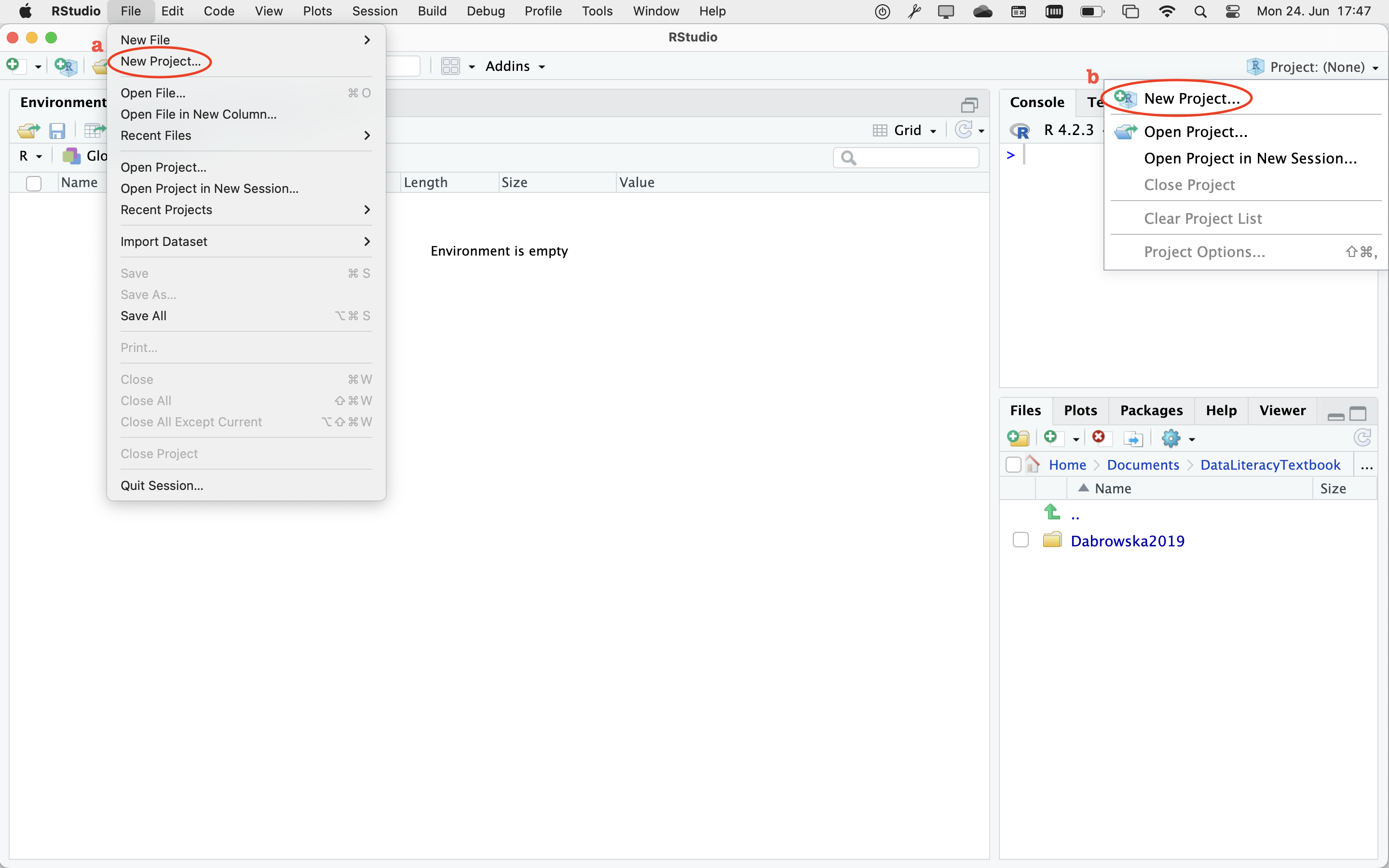
To create a new Project, you have two options. In RStudio, you can select ‘File’, then ‘New Project…’ (see Figure 6.1 a). Alternatively, you can click on the Project button in the top-right corner of your RStudio window and then select ‘New Project…’ (see Figure 6.1 b).
Both options will open up a window with three options for creating a new project:
- New Directory (which allows you to create an entirely new project for which you do not yet have a folder on your computer)
- Existing Directory (which allows you to create a project in an existing folder associated with your project)
- Version Control (see Bryan n.d.).
In Section 6.2, you should have already saved the data that we want to import in a dedicated folder on your computer. Here, a folder is the same as a directory. Hence, you can select the second option: ‘Existing Directory’.
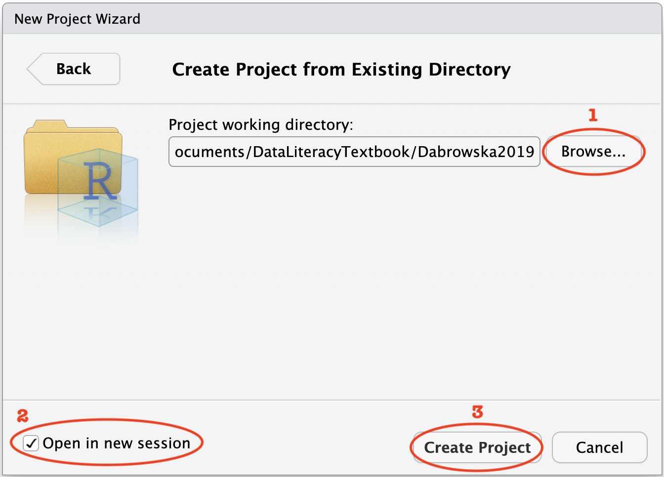
Clicking on this option will open up a new window (Figure 6.2). Click on ‘Browse…’ to navigate to the folder where you intend to save all your work related to Dąbrowska (2019). If you followed my suggestions earlier on, this would be a folder called something along the lines of Dabrowska2019. Once you have selected the correct folder, select the option ‘Open in a new session’ and then click on ‘Create Project’.
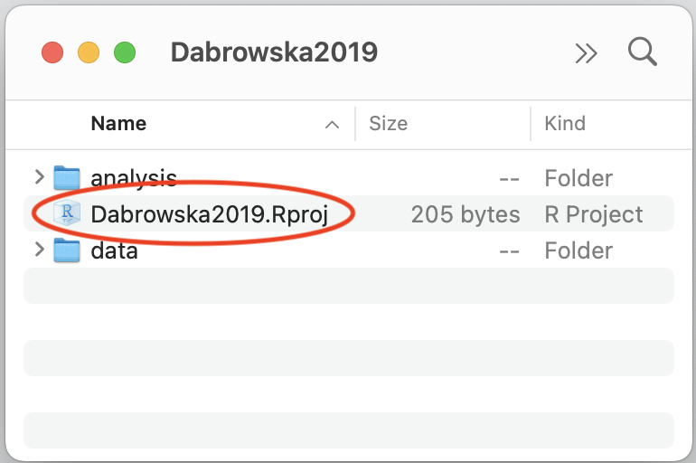
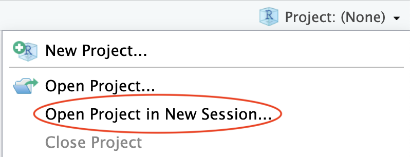
Creating an RStudio project generates a new file in your project folder called Dabrowska2019.Rproj. You can see it in the Files pane of RStudio. Note that the extension of this newly created file is .Rproj. Such .Rproj files store information about your project options, which you will not need to edit. More usefully, .Rproj files can be used as shortcuts for opening your projects. To see how this works, shut down RStudio. Then, in your computer file system (e.g. using a File Explorer window on Windows and a Finder window on macOS), navigate to your project folder to locate your .Rproj file (see Figure 6.3 (a)). Double-click on the file. This will automatically launch RStudio with all the correct settings for this particular project. Alternatively, you can use the Project button in the top-right corner of your RStudio window to open up a project from RStudio itself (see Figure 6.3 (b)).
6.4 Working directories
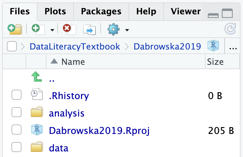
The folder in which the .Rproj file was created corresponds to your project’s working directory. Once you have opened a Project, you can see the path to your project’s working directory at the top of the Console pane in RStudio. The Files pane should also show the content of this directory as in Figure 6.4.
Click on the “New Folder” icon in your Files pane to create a new subfolder called analysis. Your folder Dabrowska2019 should now contain an .RProj file and two subfolders called analysis and data.
6.5 Importing data from a .csv file
We will begin by creating a new R script in which we will write the code necessary to import the data from Dąbrowska (2019)‘s study in R. To do so, from the Files pane in RStudio, click on the analysis folder to open it and then click on the ’New Blank File’ icon in the menu bar of the Files pane and select ‘R Script’. This will open a new, empty R script in your Source pane. It is best to always begin by saving a newly created file. Save this empty script with a computer- and human-friendly file name such as 1_DataImport.R (Section 3.2). It should now appear in your analysis folder in the Files pane.
Given that we want to import two .csv files, we are going to use the function read.csv(). You can find out what this function does by running the command ?read.csv or help(read.csv) in the Console to open up the documentation. This help file contains information about several base R functions used to import data. Scroll down to find the information about the read.csv() function. It reads:
read.csv(file, header = TRUE, sep = ",", quote = "\"",
         dec = ".", fill = TRUE, comment.char = "", ...)
This line from the documentation informs us that this function’s first argument is the path to the file from which we want to import the data. It also informs us that file is the only argument that does not have a default value (as it is not followed by an equal sign and a value). In this function, file is therefore the only argument that is compulsory. Hence, in theory, all we need to write to import the data is:
L1.data <- read.csv(file = "data/L1_data.csv")In fact, we could shorten things even further as, unless otherwise specified, R will assume that the first value listed after a function corresponds to the function’s first argument which, here, is file. In other words, this command and the one above are equivalent:
L1.data <- read.csv("data/L1_data.csv")The file path "data/L1_data.csv" informs R that the data are located in a subfolder of the project’s working directory called data and that, within this data subfolder, the file that we want to import is called L1_data.csv. Note that the file extension must be specified (see Section 2.3). Note, also, the file path is separated with a single forward slash /. In R, this should work regardless of the operating system that you are using and, in order to be able to easily share your scripts with others, it is recommended that you use forward slashes even if you are running Windows (Section 3.3).
Although the command above did the job, in practice, it is often safer to spell things out further to remind ourselves of some of the default settings of the function that we are using in case they need to be checked or changed at a later stage. In this example, we will therefore import the data with the following command:
L1.data <- read.csv(file = "data/L1_data.csv",
                    header = TRUE,
                    sep = ",",
                    quote = "\"",
                    dec = ".")
In the command above, header = TRUE, explicitly tells R to import the first row of the .csv table as column headers rather than values. This is not strictly necessary because, as we saw from the function’s help file, TRUE is already set as the default value for this argument, but it is good to remind ourselves of how this particular dataset is organised.
The arguments sep and quote specify the characters that, in this .csv file are used to separate the values on the one hand, and delineate them, on the other (see Section 2.5.1). As we saw above, Dąbrowska (2019)’s .csv files use the comma as the separator and the double quotation mark as the quoting character. Note that the " character needs to be preceded by a backslash (\) (we say it needs to be “escaped”) because otherwise R will interpret it as part of the command syntax, which would lead to an error. Finally, the argument dec = "." explicitly tells R that this .csv file uses the dot as the decimal point. In some countries, e.g. Germany and France, the comma is used to represent decimal places so, if you obtain data from a German or French colleague, this setting may need to be changed to dec = "," for the data to be imported correctly.
This section title borrows a quote from The Tempest by William Shakespeare to reflect the fact that file paths are perhaps the most frequent source of frustration among (beginner) coders. Section 6.6 explains how to deal with the most frequent error messages. Ultimately, however, these errors are typically due to poor data management (see Chapter 3). That’s because the devil’s in the detail (remember: no spaces, special characters, differences between different operating systems, etc.). As a result, even advanced users of R and other programming languages frequently find that file path issues continue to plague their work, if they fail to take file management seriously.
To make your projects more robust to such issues, I strongly recommend working with the {here} package in addition to R Projects. You will first need to install the package:
install.packages("here")When you load the package, it automatically runs the here() function with no argument, which returns the path to your project directory, as determined by the location of the .RProj file associated with your project.
library(here)You can now use the here() function to build paths relative to this directory with the following syntax:
here("data", "L1_data.csv")[1] "/Users/lefoll/Documents/UzK/RstatsTextbook/data/L1_data.csv"And you can embed this path in your import command like this:
library(here)

L1.data <- read.csv(file = here("data", "L1_data.csv"))
Much like wearing a helmet for extra safety (Figure 6.5), {here} makes the paths that you include in your code far more robust. In other words, they are far less likely to fail and break your code when you share your scripts with your colleagues, or run them yourself from different directories or operating systems. For more reasons to use {here}, check out Malcolm Barrett (2018)’s blog post “Why should I use the here package when I’m already using projects?”.
Although a fairly common way of working with data in R, using setwd() (see Section 6.12.1) is dangerous and will, sooner or later, cause you and/or your colleagues some nasty accidents (see Figure 6.5). A combination of using R projects (.RProj) and the {here} package as described above is much safer!
6.6 Import errors and issues 🥺
It is crucial that you check whether your data have genuinely been correctly imported. Here’s a list of things to check (in that order):
Were you able to run the import command without producing any errors? If you are getting an error, remember that this is most likely due to a typo (see Section 5.6)!
If part of the error message reads “No such file or directory”, this means that either the file path or the file name is incorrect. Carefully check the path that you specified in your import command (if you’re struggling to find the correct path, you may want to try out the import method explained in Section 6.12.2). To ensure that you are not misspelling the name of the file, you can press the
tabkey on your keyboard to get RStudio to auto-complete the file name for you.If the error message includes the statement “could not find function”, this means that you have either misspelled the name of the function or this is not a base
Rfunction and you have forgotten to load the library to which this function belongs (see Section 6.8).As usual whenever you get an error message, also check that you have included all of the necessary brackets and quotation marks (see Section 5.6).
Has the
Rdata object appeared in your Environment pane? Does it have the expected number of rows (observations) and columns (variables)?L1.datacontains 90 observations and 31 variables. If you are getting different numbers, this might be because you previously opened the.csvfile with Excel or that your computer converted it to Excel format automatically. To remedy this, ensure that you have followed all the steps described in Section 2.5.2.To view the entire table, use the function
View()with the name of your data object as the first and only argument, e.g.View(L1.data). This will open up a new tab in your Source pane that displays the full table, much like in a spreadsheet programme. You can search and filter the table in this tab, but you cannot edit it in any way (and that’s a good thing because, if we want to edit things, we want to ensure that we keep track of our changes in a script!). Browse through the table and check that everything “looks healthy”. This is much like visually inspecting and smelling ingredients before using them in a recipe. It’s not perfect but if something is really off, you should notice it. Check that each cell appears to have one and only one value.Finally, use the
str()function to view the structure of your data object in a more compact way. Using the commandstr(L1.data)will display a summary of the data.frame in the Console. The summary begins by informing us that this data object is a data.frame, that contains 90 observations and 31 variables. Then, it lists all of the variables, followed by the type of values stored in this variable (e.g. character strings or integers) and then the first few values for each variable. Especially with very wide tables that contain a lot of variables, it is often easier to check the summary of the imported data withstr()than withView(), though I would always recommend taking a few seconds to do both. This is time well spent!
Rs!
Note that, unlike the functions that we have used so far, the View() function begins with a capital letter. R is a case-sensitive programming language, which means that view() and View() are not the same thing!
Import both data files from Dąbrowska (2019) using the read.csv function as described above. Save the first as the R object L1.data (as in the example above) and the second as L2.data. Then, answer the following questions.
Q6.8 In the two data files from Dąbrowska (2019), each row corresponds to one participant. How many L1 participants were included in this study?
Q6.9 How many L2 participants were included in Dąbrowska (2019)’s study?
Q6.10 Compare the data frames containing the L1 and L2 data. Which dataset contains more variables?
Q6.11 You have saved the two datasets to your local R environment as L1.data and L2.data. What kind of R objects are L1.data and L2.data? You can find out by using the command class(). It simply takes the name of the object as its only argument.
Q6.12 Why does the L2 dataset contain the variable NativeLg, but not the L1 dataset?
6.7 Importing tabular data in other formats
We have seen how to load data from a .csv file into R by creating an R data frame object that contains the data extracted from a .csv file. But, as we saw in Chapter 2, not all datasets are stored as .csv files. Fear not: there are many import functions in R, with which you can import pretty much all kinds of data formats! This section introduces a few of the most useful ones for research in the language sciences.
We begin with the highly versatile function read.table(). The read.csv() is actually a variant of read.table(). You recall that when we called up the help file for the former using ?read.csv(), we obtained a combined help file for several functions, the first of which was read.table(). By specifying the following arguments as we did earlier, we can actually use the read.table() function to import our .csv file with exactly the same results:
L1.data <- read.table(file = "data/L1_data.csv",
                    header = TRUE,
                    sep = ",",
                    quote = "\"",
                    dec = ".")
6.7.1 Tab-separated file
In Task 2.3 in Section 2.5.2, you downloaded and examined a DSV file with a .txt extension that was separated by tabs: offlinedataLearners.txt from Schimke et al. (2018).
If we change the separator character argument to \t for tab, we can also import this dataset in R using the read.table() function:
OfflineLearnerData <- read.table(file = "data/offlinedataLearners.txt",
                                        header = TRUE,
                                        sep = "\t",
                                        dec = ".")
For the command above to work, you will first need to save the file offlinedataLearners.txt to the folder specified in the path. Otherwise, you will get an error message informing you that there is “No such file or directory” (see Section 6.6).
6.7.2 Semi-colon-separated file
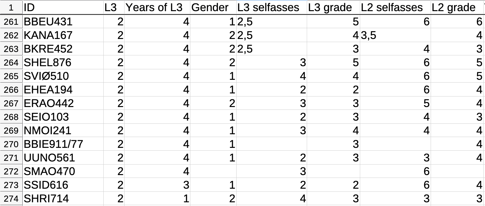
Figure 6.6 displays an extract of the dataset AJT_raw_scores_L2.csv from an experimental study by Busterud et al. (2023). Although this DSV file has a .csv extension, it is actually separated by semicolons. As you can see in Figure 6.6, in the file AJT_raw_scores_L2.csv, the comma is used to show the decimal place.
If you look carefully, you will also see that this dataset has some empty cells. These data can be downloaded from https://doi.org/10.18710/JBMAPT. It is delivered with a README text file. It is good practice to include a README file when publishing datasets or code and, as the name suggests, it is always a good idea to actually read README files! :upside-down-face: Among other things, this particular README explains that, in this dataset: “Missing data are represented by empty cells.”
If you call up the help file for the read.table() function again, you will see that there is an argument called na.strings. The default value is NA. When we import this dataset AJT_raw_scores_L2.csv from Busterud et al. (2023), we will therefore need to change this argument to ensure that empty cells are recognised as missing values.
In addition to the file path, the command to import this dataset specifies the separator character as the semicolon (sep = ";"), the character used to represent decimals (dec = ","), and empty cells as missing values (na.strings = ""):
AJT.raw.scores.L2 <- read.table(file = "data/AJT_raw_scores_L2.csv",
                          header = TRUE,
                          sep = ";",
                          dec = ",",
                          na.strings = "")
Once we have run this command, we should check that the data have been correctly imported, for example by using the View() function:
View(AJT.raw.scores.L2) ID L3 Years.of.L3 Gender L3.selfasses L3.grade L2.selfasses L2.grade
1 BKRE452 2 4 2 2.5 3 4 3
2 SHEL876 2 4 2 3.0 5 6 5
3 SVIØ510 2 4 1 4.0 4 6 5
4 EHEA194 2 4 1 2.0 2 6 4
5 ERAO442 2 4 2 3.0 3 5 4
6 SEIO103 2 4 1 2.0 3 4 3Here, we can see that the data have been correctly imported as a table. The commas have been correctly converted to decimal points and the empty cells are now labelled NA.
6.8 Using {readr} to import tabular files
The {tidyverse} is a family of packages that we will use a lot in future chapters (see Section 9.1). This family of package includes the {readr} package which features some very useful functions to import data into R. You can install and load the {readr} package either individually or as part of the {tidyverse} bundle:
- 1
- Install just this package
- 2
- Or install the full tidyverse (this will take a little longer).
- 3
- Load the library.
6.8.1 Delimiter-separated values (DSV) files
The {readr} package includes functions to import DSV files that are similar, but not identical to the base R functions explained above. The main difference is that the {readr} functions load data into an R object of type “tibble” rather than “data frame”. In practice, this will not make a difference for our work in future chapters. Hence, the following two commands can equally be used to import L1_data.csv:
- 1
-
Import
.csvfile using the baseRfunctionread.csv() - 2
-
Import
.csvfile using the {readr} functionread_csv()
[1] "data.frame"
[1] "spec_tbl_df" "tbl_df"      "tbl"         "data.frame"
Note that instead of the argument header = TRUE, the {readr} function read_csv() takes the argument col_names = TRUE, which has the same effect. There are a few more differences between the two functions that are worth noting:
- If the column headers in your original data file contain spaces, these will be automatically replaced by dots (
.) when you import data using baseRfunctions. By contrast, with the {readr} functions, the spaces will, by default, be retained. As we will see later, this behaviour can represent both an advantage and disadvantage, depending on what you want to do. - The {readr} functions are quicker and are therefore recommended if you are importing large datasets.
- In general, the behaviour of {readr} functions is more consistent across different operating systems and locale settings (e.g. the language in which your operating system is set).
Note that, just like read.csv() was a special case of read.table, the {readr} function read_csv() is a special variant of the more general function read_delim() that can be used to import data from all kinds of DSV files. Check the help file to find out all the options using ?read_delim. The help file informs us that the package includes a function specifically designed to import semi-colon separated file with the the comma as the decimal point: read_csv2(). It further states that “[t]his format is common in some European countries.” If you scroll down the help page, you will see that its usage is summarised in the following way:
read_csv2(
  file,
  col_names = TRUE,
  col_types = NULL,
  col_select = NULL,
  id = NULL,
  locale = default_locale(),
  na = c("", "NA"),
  quoted_na = TRUE,
  quote = "\"",
  comment = "",
  trim_ws = TRUE,
  skip = 0,
  n_max = Inf,
  guess_max = min(1000, n_max),
  progress = show_progress(),
  name_repair = "unique",
  num_threads = readr_threads(),
  show_col_types = should_show_types(),
  skip_empty_rows = TRUE,
  lazy = should_read_lazy()
)
This overview of the read_csv2 function shows all of the arguments of the function and their default values. For instance, with na = c("", "NA"), it tells us that, by default, both empty cells and cells with the value NA will be interpreted by the function as NA values.
Having checked the default values for all of the arguments of the read_csv2 function, we may conclude that we can safely use this {readr} function to import the file AJT_raw_scores_L2.csv from Busterud et al. (2023) without changing any of these default values. Hence, all we need is:
AJT.raw.scores.L2 <- read_csv2(file = "data/AJT_raw_scores_L2.csv")Note that, whereas when we used the base R function read.table() the header for the third variable in the file was imported as Years.of.L3, using the {readr} function, the variable is entitled Years of L3.
6.8.2 Fixed-width files
Fixed-width files (with file extensions such as .gz, .bz2 or .xz) are a less common type of data source in the language sciences. In these text-based files, the values are separated not by a specific character such as the comma or the tab, but by a set amount of white/empty space other than a tab. Fixed-width files can be loaded using the read_fwf() function from {readr}. Fields can be specified by their widths with fwf_widths() or by their positions with fwf_positions().
6.9 Importing files from spreadsheet software
If your data are currently stored in a spreadsheet software (e.g. LibreOffice Calc, Google Sheets, or Microsoft Excel), you can export them to .csv or .tsv, which are better archiving and sharing formats. However, if you do not wish to do this (e.g. because your colleague wishes to maintain the spreadsheet format that includes formatting elements such as bold or coloured cells) or because this is not your own data, you’ll be pleased to learn that there are functions to import these file formats directly into R.
6.9.1 LibreOffice/OpenOffice Calc
To import .ods files, as used natively by open-source text processing software such as LibreOffice Calc (which you should have installed in Section 1.2) and OpenOffice Calc, you can install the {readODS} package and use its read_ods() function:
- 1
- Install from CRAN. This is the safest option.
- 2
- Alternatively, install the development version from Github.
- 3
- Load the library.
- 4
-
Import the first tab of your
.odsspreadsheet, ensuring that the first row is processed as the column headers and thatNAare recognised as such.
6.9.2 Microsoft Excel
Various packages can be used to import Microsoft Excel file formats, but the simplest is {readxl}, which is also part of the {tidyverse} (Section 9.1). It allows users to import data in both .xlsx and the older .xls format.
- 1
- Install from CRAN (safest option).
- 2
- Or install the development version from Github.
- 3
- Load the library.
- 4
-
Import the first tab of your Excel spreadsheet, ensuring that the first row is processed as the column headers and that
NAare recognised as such.
6.9.3 Google Sheets
There are also several ways to import data from Google Sheets. The simplest is to export your tabular data as a .csv, .tsv, .xslx, or .ods file by selecting Google Sheet’s menu option under ‘File’ and ‘Download’. Then, you can import this downloaded file in R using the corresponding function as described above.
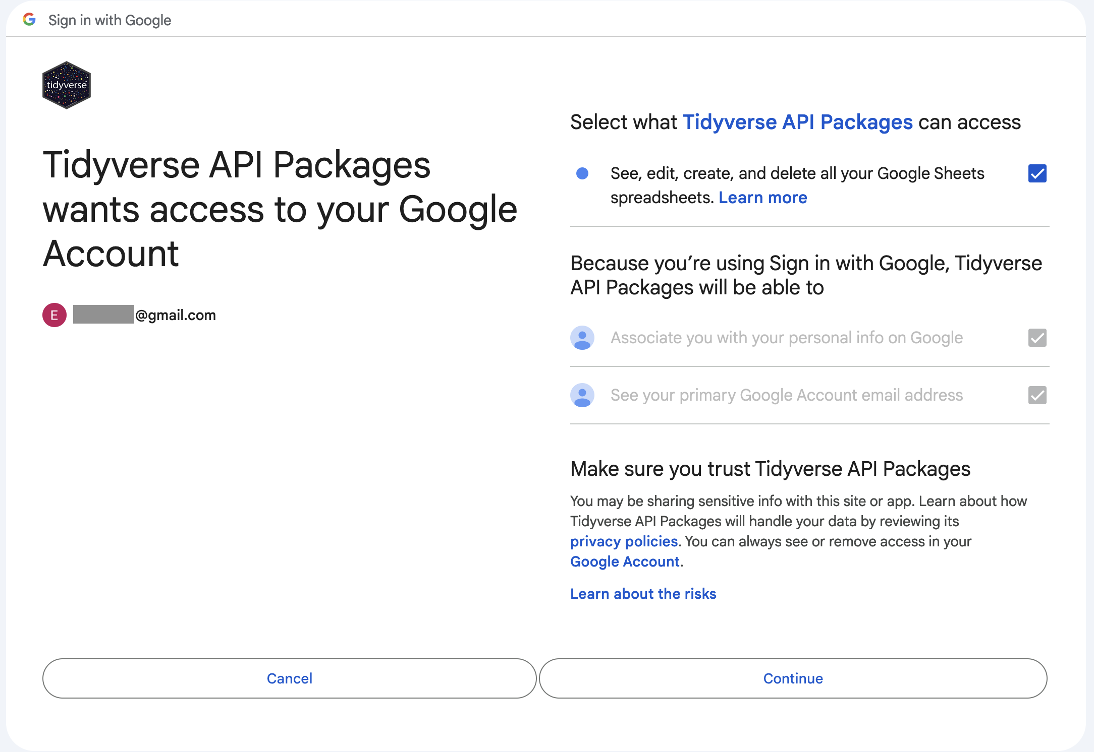
However, if you want to directly import your data from Google Sheets and be able to dynamically update the analyses that you conduct in R even as the input data are amended on Google Sheets, you can use the {googlesheets4} package (which is part of the {tidyverse}):
1install.packages("googlesheets4")
2remotes::install_github("tidyverse/googlesheets4")

3library(googlesheets4)

4MySheetsData <- read_sheet("https://docs.google.com/spreadsheets/YourURL",
                            sheet = 1,
                            col_names = TRUE,
                            na = "NA")

5MySheetsData <- read_sheet("YourGoogleSheetsID",
                            sheet = 1,
                            col_names = TRUE,
na = "NA")- 1
- Install from CRAN (safest option).
- 2
- Or install the development version from Github.
- 3
- Load the library.
- 4
- Import your Google Sheets data using its URL.
- 5
- Or import your Google Sheets data using just the sheet’s ID.
Note that, as spreadsheet software typically allow users to have several “sheets” or “tabs” within a file that each contains separate tables, the functions read_excel(), read_ods(), and read_sheet include an argument called sheet which allows you to specify which sheet should be imported. The default value is 1, which simply means that the first one is imported. If your sheets have names, you can also use its name as the argument value, e.g.:
MyExcelData <- read_excel("data/MyExcelSpreadsheet.xlsx",
                            sheet = "raw data",
                            col_names = TRUE,
                            na = NA)
6.10 Importing data files from SPSS, SAS and Stata
If you’ve recently switched from working in SPSS, SAS, or Stata (or are collaborating with someone who uses these programmes), it might be useful to know that you can also import the data files created by programmes directly into R using the {haven} package.
- 1
- Install from CRAN (safest option).
- 2
- Or install the development version from Github.
- 3
- Load the library.
- 4
- Import a SAS data file.
- 5
- Import a SPSS data file.
- 6
- Import a Stata data file.
6.11 Importing other file formats
In this textbook, we will only deal with DSV files (Section 2.5.1) but, as you can imagine, there are many more R packages and functions that allow you to import all kinds of other file formats. These include .xml, .json and .html files, various database formats, and other files with complex structures (see, e.g. https://rc2e.com/inputandoutput).
In addition, fellow linguists are constantly developing new packages to work with file formats that are specific to our discipline. In the spirit of Open Science (see Chapter 1), many are making these packages available to the wider research community by releasing them under open licenses. For example, linguistics M.A. students Katja Wiesner and Nicolas Werner wrote and published an R package called rELAN to facilitate the import of the .eaf files generated by the linguistics annotation software ELAN (Lausberg & Sloetjes 2009) as part of a seminar project supervised by Dr. Fahime (Fafa) Same at the University of Cologne.
6.12 Quick-and-dirty (aka bad!) ways to import data in R
Feel free to skip this section if you got on just fine with the importing method introduced above as the following two methods are problematic for a number of reasons. However, they may come in useful in special cases and you will certainly find scripts that include hardcoded paths, which is why both are briefly explained below.
6.12.1 Hardcoding file paths in R scripts 🥴
Whilst it is certainly not recommended (see e.g. Bryan 2017), it is nonetheless worth understanding this method of working with file paths in R as you may well come across it in other people’s code.
Instead of creating an R Project to determine a project’s working directory (as we did in Section 6.3), it is possible to begin a script with a line of code that sets the working directory for the script using the function setwd(), e.g.:
setwd("/Users/lefoll/UzK/RstatsTextbook/Dabrowska2019")Afterwards, data files can be imported using a relative path from the working directory just like we did earlier.
L1.data <- read.csv(file = "data/L1_data.csv")If you have to work with an R script that uses this method, you will need to amend the path designated as the working directory by setwd() to the corresponding path on your own computer. This might not sound like much of an issue, but as data scientist, R expert, and statistics professor Jenny Bryan (2017) explains:
The chance of the
setwd()command having the desired effect – making the file paths work – for anyone besides its author is 0%. It’s also unlikely to work for the author one or two years or computers from now. The project is not self-contained and portable.
In the language sciences, not everyone is aware of the severity of these issues. Hence, it is not uncommon for researchers to make their scripts even less reproducible by not setting a working directory at all and, instead, relying exclusively on absolute paths (Section 3.3). Hence, every time they want to import data (and, as we will see later on, export objects from R, too), they write out the full file path in the command like this:
L1.data <- read.csv(file = "/Users/lefoll/Documents/UzK/RstatsTextbook/Dabrowska2019/data/L1_data.csv")Having to work with such a script is particularly laborious because it means that, if you inherit such a script from a colleague, you will have to manually change every single file path in the script to the corresponding file paths on your own computer. And, as Bryan (2017) points out, this will also apply if you change anything in your own computer directory structure! I hope I’ve made clear that the potential for making errors in the process is far too important to even consider going down that route.
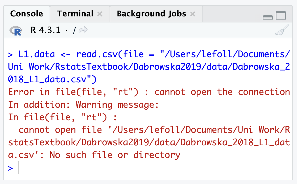
However, should you have to use this method at some point for whatever reason, you can make use of Section 3.3 which explained how to copy full file paths from a file Explorer or Finder window. Note that if there are spaces or other special characters other than _ or - anywhere in your file path, your import command will fail (see Section 3.2 on naming conventions for folders and files). The import command in Figure 6.8, for instance, fails and returns an error (see ) because the folder “Uni Work” contains a space.
The only way to fix this issue is to remove the space in the name of the folder (in your File Finder or Navigator window) and then amend the file path in your R script accordingly.
6.12.2 Importing data using RStudio’s GUI :face-with-rolling-eyes:
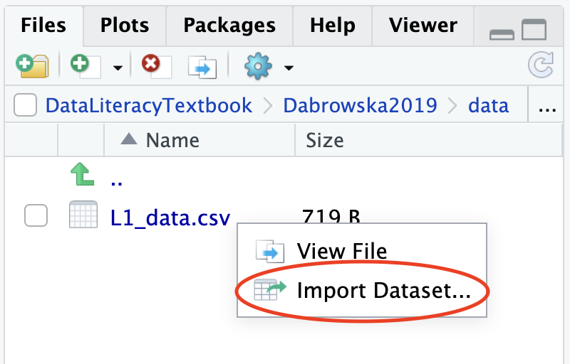
You may have noticed that, if you click on a data file from the Files pane in RStudio (Figure 6.9), RStudio will offer to import the dataset for you. This looks like (and genuinely is) a very convenient way to import data in an R session using RStudio’s GUI (graphical user interface).
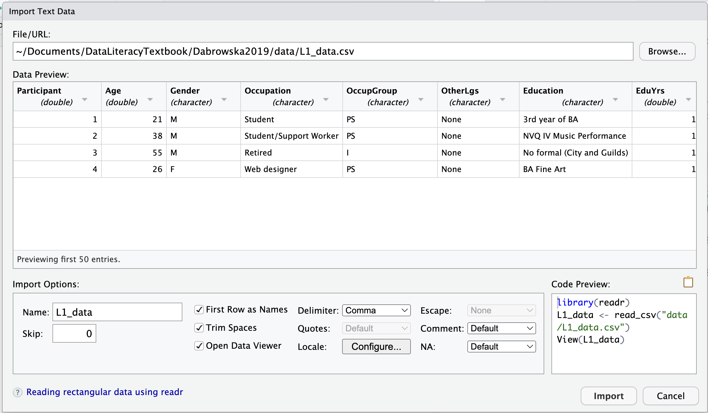
Clicking on “Import Dataset” opens up RStudio’s “Import Text Data” dialogue box, which is similar to the one that we saw in LibreOffice Calc (Section 2.5.2). It allows you to select the relevant options to correctly import the file and displays a preview to check that the options that you have selected are correct. You can also specify the name of the R object to which you want to assign the imported data. By default, the name of the data file (minus the file extension and any special characters) is suggested.
As soon as you click on the ‘Import’ button, the data are imported and opened using the View() function for you to check the sanity of the data.
This importing method works a treat, so what’s not to like? Well, the first problem is that you are not in full control. You cannot select which import function is used; RStudio decides for you. You may have noticed that it chooses to use the {readr} import functions, rather than the base R ones. There are lots of good reasons to use the {readr} functions (see Section 6.8), but it may not be what you wanted to do. When we do research, it is important for us to be in control of every step of the analysis process.
Second, your data import settings are not saved in an .R script as the commands were only sent to the Console: they are part of your script. This means that if you import your data in this way, do some analyses, and then close RStudio, you will have no way of knowing with which settings you imported the data to obtain the results of your analysis! This can have serious consequences for the reproducibility of your work.
Whilst there is no way of remedying the first issue, the second can easily be fixed. After you have successfully imported your data from RStudio’s Files pane, you can (and should!) immediately copy the import commands from the Console into your .R script. In this way, the next time you want to re-run your analysis, you can begin by running these import commands directly from your .R script rather than by via RStudio’s Files pane.
If you are running into errors due to incorrect file paths, it can be useful to try to import your data using RStudio’s GUI to see where you are going wrong by comparing your own attempts with the import commands that RStudio generated.
Check your progress 🌟
You have successfully completed 0 out of 12 questions in this chapter.
Are you confident that you can…?
Now it’s time to start exploring research data in R! In Chapter 7 you will learn how to work with in-built R functions to find out more about the DSV data from Dąbrowska (2019) that you imported in this chapter.
For more on reproductions and replications, see Section 14.2.↩︎
Digital Object Identifiers (DOI) are alpha-numeric strings that can be assigned to publications, preprints, datasets, and all other kinds of research materials with the aim of facilitating the exchange of information on digital networks and avoiding dead links (Parsons et al. 2022).↩︎
