7  VaRiables and functions

Chapter overview

In this chapter, you will learn how to:

• Use base R functions to inspect a dataset
• Inspect and access individual variables from a dataset
• Access individual data points from a dataset
• Use simple base R functions to describe variables
• Look up and change the default arguments of functions
• Combine functions using two methods

WarningPrerequisites

In this chapter and the following chapters, all analyses are based on data from Dąbrowska (2019). You will only be able to reproduce the analyses and answer the quiz questions if you have created an RProject and saved the data within the project directory. Detailed instructions to do so can be found from Section 6.3 to Section 6.5.

Alternatively, you can download Dabrowska2019.zip from the textbook’s GitHub repository. To launch the project correctly, first unzip the file and then double-click on the Dabrowska2019.Rproj file.

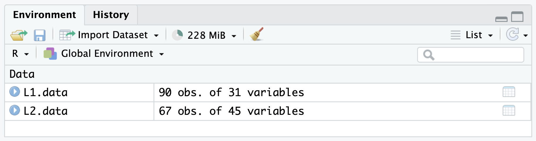
Before we get started, import both L1 and the L2 datasets to your local R environment:

library(here)

L1.data <- read.csv(file = here("data", "L1_data.csv"))
L2.data <- read.csv(file = here("data", "L2_data.csv"))

Check the Environment pane in RStudio to ensure that everything has gone to plan (see Figure 7.1).

Figure 7.1: Environment pane of RStudio showing that the datasets have been correctly loaded and are ready to be used in the current R session

7.1 Inspecting a dataset in R

In Section 6.6, we saw that we can use the View() function to display tabular data in a format that resembles that of a spreadsheet programme (see Figure 7.2).

The two datasets from Dąbrowska (2019) are both long and wide so you will need to scroll in both directions to view all the data. RStudio also provides a filter option and a search tool (see Figure 7.2). Note that both of these tools can only be used to visually inspect the data. You cannot alter the dataset in any way using these tools. And that’s a good thing because any changes that we make should be documented in code (as we will learn in Chapter 9).

View(L1.data)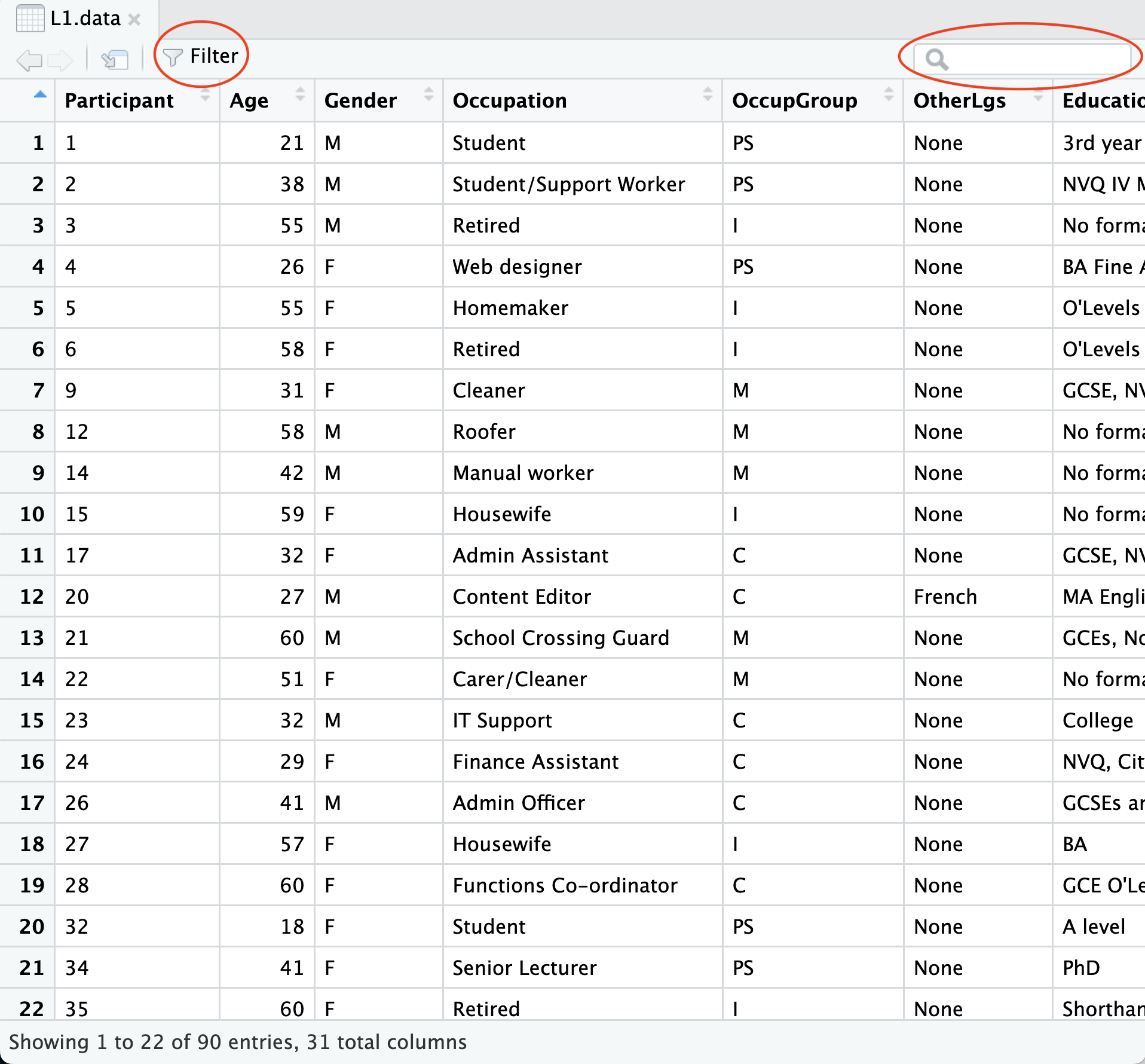

Figure 7.2: The L1.data object as visualised using the View() function in RStudio

TipYour turn!

Q7.1 The View() function is more user-friendly than attempting to examine the full table in the Console. Try to display the full L2.dataset in the Console by using the command L2.data which is shorthand for print(L2.data). What happens?

R produces an error message because there are too many rows and the Console window is not long enough.
The R Console prints the data in a randomly jumbled way.
R only displays the first 22 rows and the columns are not aligned because the Console window is not wide enough.
The R Console prints out all the data, but not the column headers.

🐭 Click on the mouse for a hint.

In practice, it is often useful to printing subsets of a dataset in the Console to quickly check the sanity of the data. To do so, we can use the function head() that prints the first six rows of a tabular dataset.

head(L1.data)

  Participant Age Gender             Occupation OccupGroup OtherLgs
1           1  21      M                Student         PS     None
2           2  38      M Student/Support Worker         PS     None
3           3  55      M                Retired          I     None
4           4  26      F           Web designer         PS     None
5           5  55      F              Homemaker          I     None
6           6  58      F                Retired          I     None
                    Education EduYrs ReadEng1 ReadEng2 ReadEng3 ReadEng Active
1              3rd year of BA     17        1        2        2       5      8
2    NVQ IV Music Performance     13        1        2        3       6      8
3 No formal (City and Guilds)     11        3        3        4      10      8
4                 BA Fine Art     17        3        3        3       9      8
5                    O'Levels     12        3        2        3       8      8
6                    O'Levels     12        1        1        2       4      8
  ObjCl ObjRel Passive Postmod Q.has Q.is Locative SubCl SubRel GrammarR
1     8      8       8       8     8    6        8     8      8       78
2     8      8       8       8     8    7        8     8      8       79
3     8      8       8       8     7    8        8     8      8       79
4     8      8       8       8     8    8        8     8      8       80
5     8      8       8       8     8    7        8     8      8       79
6     5      1       8       8     7    6        7     8      8       66
  Grammar VocabR    Vocab CollocR Colloc Blocks ART LgAnalysis
1    95.0     48 73.33333      30 68.750     16  17         15
2    97.5     58 95.55556      35 84.375     11  31         13
3    97.5     58 95.55556      31 71.875      5  38          5
4   100.0     53 84.44444      37 90.625     20  26         15
5    97.5     55 88.88889      36 87.500     16  31         14
6    65.0     48 73.33333      21 40.625      8  15          3

TipYour turn!

Q7.2 Six is the default number of rows printed by the head() function. Have a look at the function’s help file using the command ?head to find out how to change this default setting. How would you get R to print the first 10 lines of L2.data?

head(L2.data, n = 10)
head(L2.data, L = 10)
head(L2.data, rows = 10)
head(L2.data n = 10L)
head(L2.data, 10)
head(L2.data, n = 10L)

🐭 Click on the mouse for a hint.

7.2 Working with variables

7.2.1 Types of variables

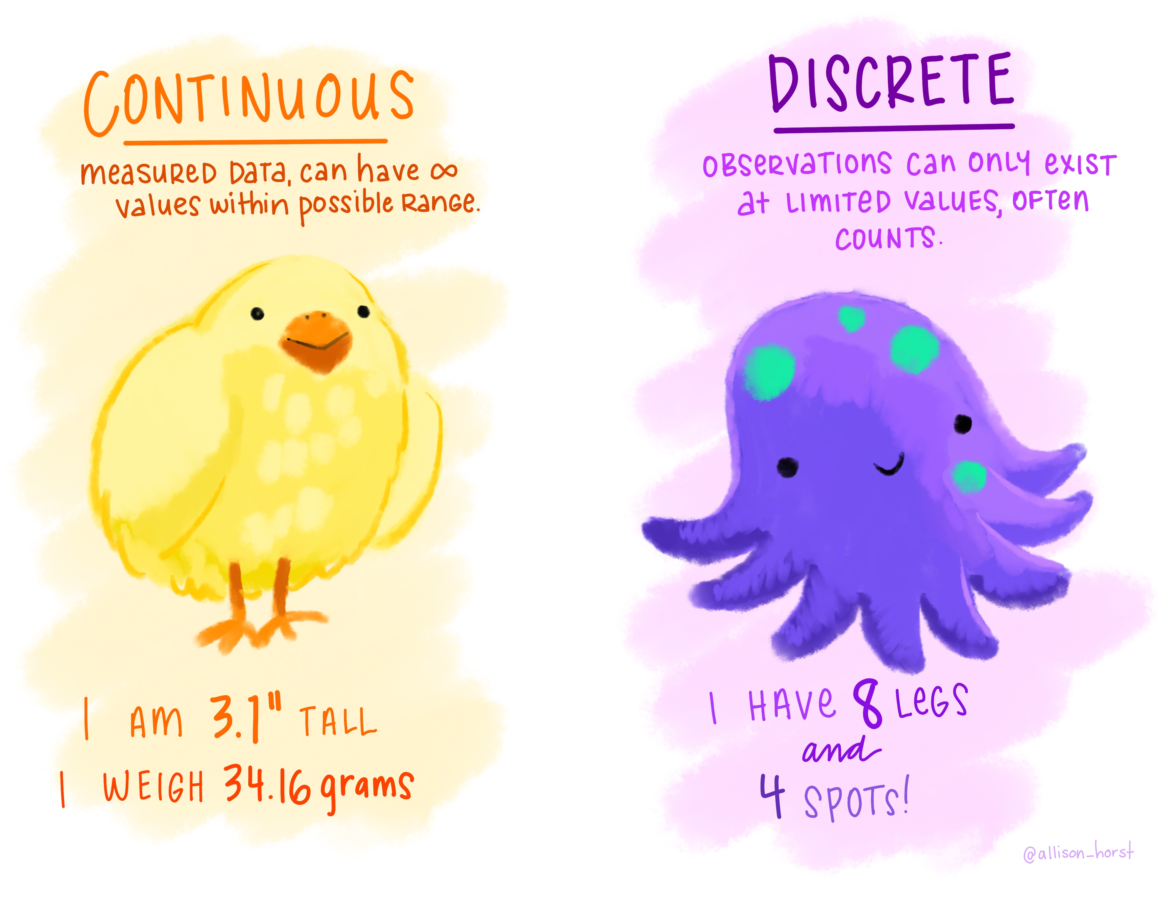
In statistics, we differentiate between numeric (or quantitative) (see Figure 7.3) and categorical (or qualitative) (see Figure 7.4) variables. Each variable type can be subdivided into different subtypes. It is very important to understand the differences between these types of data as we frequently have to use different statistics and visualisations depending on the type(s) of variable(s) that we are dealing with.

Some numeric variables are continuous: they contain measured data that, at least theoretically, can have an infinite number of values within a range (e.g. time). In practice, however the number of possible values depends on the precision of the measurement (e.g. are we measuring time in years, as in the age of adults, or milliseconds, as in participants’ reaction times in a linguistic experiment). Numeric variables for which only a defined set of values are possible are called discrete variables (e.g. number of occurrences of a word in a corpus). Most often, discrete numeric variables represent counts of something.

Figure 7.3: Numeric variables (artwork CC BY 4.0 @allison_horst)

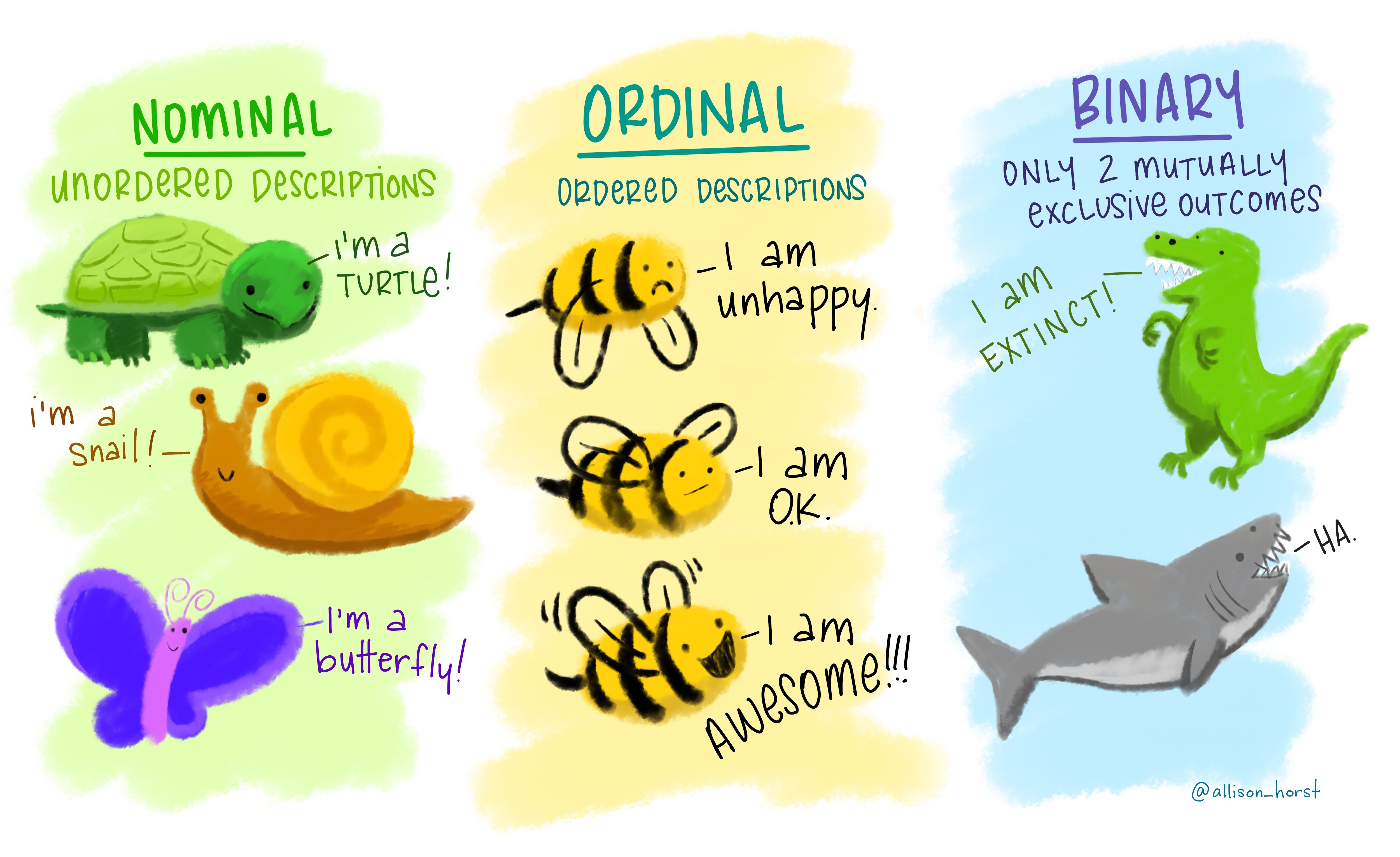
Categorical variables can be nominal or ordinal. Nominal variables contain unordered categorical values (e.g. participants’ mother tongue or nationality), whereas ordinal variables have categorical values that can be ordered meaningfully (e.g. participants’ proficiency in a specific language where the values beginner, intermediate and advanced or A1, A2, B1, B2, C1 and C2 have a meaningful order). However, the difference between each category (or level) is not necessarily equal. Binary variables are a special case of nominal variable which only has two mutually exclusive outcomes (e.g. true or false in a quiz question).

Figure 7.4: Categorical variables (artwork CC BY 4.0 @allison_horst)

TipYour turn!

Q7.3 Which type of variable is stored in the Occupation column in L1.data?

Continuous
Nominal
Other
Binary
Discrete

Q7.4 Which type of variable is stored in the Gender column in L1.data?

Nominal
Continuous
Discrete
Other
Binary

Q7.5 Which type of variable is stored in the column VocabR in L1.data?

Discrete
Nominal
Continuous
Other
Binary

7.2.2 Inspecting variables in R

In tidy data tabular formats (see Chapter 8), each row corresponds to one observation and each column to a variable. Each cell, therefore, corresponds to a single data point, which is the value of a specific variable (column) for a specific observation (row). As we will see in the following chapters, this data structure allows for efficient and intuitive data manipulation, analysis, and visualisation.

The names() functions returns the names of all of the columns of a data frame. Given that the datasets from Dąbrowska (2019) are ‘tidy’, this means that names(L1.data) returns a list of all the column names in the L1 dataset.

names(L1.data)

 [1] "Participant" "Age"         "Gender"      "Occupation"  "OccupGroup" 
 [6] "OtherLgs"    "Education"   "EduYrs"      "ReadEng1"    "ReadEng2"   
[11] "ReadEng3"    "ReadEng"     "Active"      "ObjCl"       "ObjRel"     
[16] "Passive"     "Postmod"     "Q.has"       "Q.is"        "Locative"   
[21] "SubCl"       "SubRel"      "GrammarR"    "Grammar"     "VocabR"     
[26] "Vocab"       "CollocR"     "Colloc"      "Blocks"      "ART"        
[31] "LgAnalysis" 

7.2.3 R data types

A useful way to get a quick and informative overview of a large dataset is to use the function str(), which was mentioned in Section 6.6. It returns the “internal structure” of any R object. It is particular useful for large tables with many columns

str(L1.data)

'data.frame':   90 obs. of  31 variables:
 $ Participant: chr  "1" "2" "3" "4" ...
 $ Age        : int  21 38 55 26 55 58 31 58 42 59 ...
 $ Gender     : chr  "M" "M" "M" "F" ...
 $ Occupation : chr  "Student" "Student/Support Worker" "Retired" "Web designer" ...
 $ OccupGroup : chr  "PS" "PS" "I" "PS" ...
 $ OtherLgs   : chr  "None" "None" "None" "None" ...
 $ Education  : chr  "3rd year of BA" "NVQ IV Music Performance" "No formal (City and Guilds)" "BA Fine Art" ...
 $ EduYrs     : int  17 13 11 17 12 12 13 11 11 11 ...
 $ ReadEng1   : int  1 1 3 3 3 1 3 2 1 2 ...
 $ ReadEng2   : int  2 2 3 3 2 1 2 2 1 2 ...
 $ ReadEng3   : int  2 3 4 3 3 2 3 3 1 2 ...
 $ ReadEng    : int  5 6 10 9 8 4 8 7 3 6 ...
 $ Active     : int  8 8 8 8 8 8 7 8 8 8 ...
 $ ObjCl      : int  8 8 8 8 8 5 8 4 7 5 ...
 $ ObjRel     : int  8 8 8 8 8 1 8 8 3 8 ...
 $ Passive    : int  8 8 8 8 8 8 8 8 2 8 ...
 $ Postmod    : int  8 8 8 8 8 8 7 7 6 8 ...
 $ Q.has      : int  8 8 7 8 8 7 8 1 3 0 ...
 $ Q.is       : int  6 7 8 8 7 6 7 8 7 8 ...
 $ Locative   : int  8 8 8 8 8 7 8 8 8 8 ...
 $ SubCl      : int  8 8 8 8 8 8 8 8 7 8 ...
 $ SubRel     : int  8 8 8 8 8 8 8 8 7 8 ...
 $ GrammarR   : int  78 79 79 80 79 66 77 68 58 69 ...
 $ Grammar    : num  95 97.5 97.5 100 97.5 65 92.5 70 45 72.5 ...
 $ VocabR     : int  48 58 58 53 55 48 39 48 31 42 ...
 $ Vocab      : num  73.3 95.6 95.6 84.4 88.9 ...
 $ CollocR    : int  30 35 31 37 36 21 29 33 22 29 ...
 $ Colloc     : num  68.8 84.4 71.9 90.6 87.5 ...
 $ Blocks     : int  16 11 5 20 16 8 8 10 7 9 ...
 $ ART        : int  17 31 38 26 31 15 7 10 6 6 ...
 $ LgAnalysis : int  15 13 5 15 14 3 4 5 2 6 ...

At the top of its output, the function str(L1.data) first informs us that L1.data is a data frame object, consisting of 90 observations (i.e. rows) and 31 variables (i.e. columns). Then, it returns a list of all of the variables included in this data frame. Each line starts with a $ sign and corresponds to one column. First, the name of the column (e.g. Occupation) is printed, followed by the column’s R data type (e.g. chr for a character string vector), and then its values for the first few rows of the table (e.g. we can see that the first participant in this dataset was a “Student” and the second a “Student/Support Worker”).

TipYour turn!

Compare the outputs of the str() and head() functions in the Console with that of the View() function to understand the different ways in which the same dataset can be examined in RStudio.

Q7.6 Use the str() function to examine the internal structure of the L2 dataset. How many columns are there in the L2 dataset?

Q7.7 Which of these columns can be found in the L2 dataset, but not the L1 one?

FirstExp
NativeLg
OtherLgs
Arrival
EduYrs
EngWork

🐭 Click on the mouse for a hint.

Q7.8 Which type of R object is the variable Arrival stored as?

digit
string character
interest
index
integer
intelligence

🐭 Click on the mouse for a hint.

Q7.9 How old was the third participant listed in the L2 dataset when they first moved to an English-speaking country?

🐭 Click on the mouse for a hint.

Q7.10 In both datasets, the column Participant contains anonymised participant IDs. Why is the variable Participant stored as string character vector in L1.data, but as an integer vector in L2.data?

Because the L1 participants' IDs are written out as words rather than digits.
Because the L1 participants' IDs only contain whole numbers with no decimal points.
Because some of the L1 participants' IDs contain letters as well as numbers.
Because there are more L1 participants than L2 participants.

🐭 Click on the mouse for a hint.

7.2.4 Accessing individual columns in R

We can call up individual columns within a data frame using the $ operator. This displays all of the participants’ values for this one variable. As shown below, this works for any type of data.

L1.data$Gender

 [1] "M" "M" "M" "F" "F" "F" "F" "M" "M" "F" "F" "M" "M" "F" "M" "F" "M" "F" "F"
[20] "F" "F" "F" "F" "F" "F" "M" "F" "M" "F" "M" "F" "F" "F" "M" "F" "F" "M" "F"
[39] "F" "F" "F" "F" "M" "M" "F" "F" "M" "F" "F" "F" "F" "F" "F" "F" "M" "M" "M"
[58] "F" "F" "M" "M" "M" "M" "F" "M" "M" "M" "M" "M" "M" "M" "M" "F" "M" "F" "F"
[77] "M" "M" "M" "F" "F" "M" "M" "F" "F" "M" "M" "M" "F" "M"

L1.data$Age

 [1] 21 38 55 26 55 58 31 58 42 59 32 27 60 51 32 29 41 57 60 18 41 60 21 25 26
[26] 60 57 60 52 25 23 42 59 30 21 21 60 51 62 65 19 65 29 38 37 42 20 32 29 29
[51] 27 28 29 25 33 25 25 25 52 25 53 22 65 60 61 65 65 61 30 30 32 30 39 29 55
[76] 18 32 31 20 38 44 18 17 17 17 17 17 17 17 17

Before doing any data analysis, it is crucial to carefully visually examine the data to spot any problems. Ask yourself:

• Do the values look plausible?
• Are there any missing values?

Looking at the Gender and Age variables, we can see that the L1 participants declared being either ‘male’ ("M") or ‘female’ ("F"). We note that the youngest were 17 years old, which seems reasonable and we also check that no participant was improbably old. A single improbable value is likely to be the result of a data entry error, e.g. a participant or researcher accidentally entered 188 as an age, instead of 18. If you spot a whole string of improbable or outright impossible values (e.g. C, I and PS as age values!), something has likely gone wrong during the data import process (see Section 6.6).

Just like we can save individual numbers and words as R objects to our R environment, we can also save individual columns as individual R objects. As we saw in Section 5.3, in this case, the values of the variable are not printed in the Console, but rather saved to our R environment.

L1.Occupation <- L1.data$Occupation

If we want to display the content of this variable, we must print our new R object by calling it up with its name, e.g. L1.Occupation. Try it out! As listing all of the L1 participant’s jobs makes for a very long list, below, we only display the first six values using the head() function.

head(L1.Occupation)

[1] "Student"                "Student/Support Worker" "Retired"               
[4] "Web designer"           "Homemaker"              "Retired"               

7.3 Accessing individual data points in R

We can also access individual data points from a variable using the index operator: the square brackets ([]). For example, we can access the Occupation value for the fourth L1 participant by specifying that we only want the fourth element of the R object L1.Occupation.

L1.Occupation[4]

[1] "Web designer"

We can also do this from the L1.data data frame object directly. To this end, we use a combination of the $ and the [] operators.

L1.data$Occupation[4]

[1] "Web designer"

We can access a consecutive range of data points using the : operator.

L1.data$Occupation[10:15]

[1] "Housewife"             "Admin Assistant"       "Content Editor"       
[4] "School Crossing Guard" "Carer/Cleaner"         "IT Support"           

Or, if they are not consecutive, we can list the numbers of the values that we are interesting in using the combine function (c()) and commas separating each index value.

L1.data$Occupation[c(11,13,29,90)]

[1] "Admin Assistant"       "School Crossing Guard" "Dental Nurse"         
[4] "Student"              

It is also possible to access data points from a tabular R object by specifying both the number of the row and the number of the column of the relevant data point(s) using the following pattern: [row,column].

For example, given that we know that Occupation is stored in the fourth column of L1.data, we can find out the occupation of the L1 participant in the 60^th row of the dataset like this:

L1.data[60,4]

[1] "Train Driver"

All of these approaches can be combined. For example, below we access the values of the second, third, and fourth columns for the 11^th, 13^th, 29^th, and 90^th L1 participants.

L1.data[c(11,13,29,90),2:4]

   Age Gender            Occupation
11  32      F       Admin Assistant
13  60      M School Crossing Guard
29  52      F          Dental Nurse
90  17      M               Student

TipYour turn!

The following two quiz questions focus on the NativeLg variables from the L2 dataset (L2.data).

Q7.11 Use the index operators to find out the native language of the 26^th L2 participant.

Cantonese Chinese German Italian Greek Lithuanian Mandarin Polish Russian Spanish

🐭 Click on the mouse for a hint.

Q7.12 Which command(s) can you use to display only the Gender, Occupation, Native language, and Age of the last participant listed in the L2 dataset?

L2.data[-1:c(2,3,5,9)]
L2.data[67,c(2:3,5,9)]
L2.data[90,c(2:3,5,9)]
L2.data[67,c(2,3,5,9)]
L2.data[67:c(2,3,5,9)]
L2.data[67 , c(2,3,5,9)]

🦉 Hover over the owl for a hint

🐭 Click on the mouse for a second hint.

7.4 Using built-in R functions

We know from our examination of the L1 dataset from Dąbrowska (2019) that it includes 90 English native speaker participants. To find out their mean average age, we could add up all of their ages and divide the sum by 90 (see Section 8.1 for more ways to report the central tendency of a variable).

(21 + 38 + 55 + 26 + 55 + 58 + 31 + 58 + 42 + 59 + 32 + 27 + 60 + 51 + 32 + 29 + 41 + 57 + 60 + 18 + 41 + 60 + 21 + 25 + 26 + 60 + 57 + 60 + 52 + 25 + 23 + 42 + 59 + 30 + 21 + 21 + 60 + 51 + 62 + 65 + 19 + 65 + 29 + 38 + 37 + 42 + 20 + 32 + 29 + 29 + 27 + 28 + 29 + 25 + 33 + 25 + 25 + 25 + 52 + 25 + 53 + 22 + 65 + 60 + 61 + 65 + 65 + 61 + 30 + 30 + 32 + 30 + 39 + 29 + 55 + 18 + 32 + 31 + 20 + 38 + 44 + 18 + 17 + 17 + 17 + 17 + 17 + 17 + 17 + 17) / 90

[1] 37.54444

Of course, we would much rather not write all of this out! Especially, as we are very likely to make errors in the process. Instead, we can use the base R function sum() to add up all of the L1 participant’s ages and divide that by 90.

sum(L1.data$Age) / 90

[1] 37.54444

This already looks much better, but it’s still less than ideal: What if we decided to exclude some participants (e.g. because they did not complete all of the experimental tasks)? Or decided to add data from more participants? In both these cases, 90 will no longer be the correct denominator to calculate their average age! That’s why it is better to work out the denominator by computing the total number of values in the variable of interest. To this end, we can use the length() function, which returns the number of values in any given vector.

length(L1.data$Age)

[1] 90

We can then combine the sum() and the length() functions to calculate the participants’ average age.

sum(L1.data$Age) / length(L1.data$Age)

[1] 37.54444

Base R includes lots of useful functions to do statistics, which means that it includes a built-in function to calculate mean average values. It is called mean() and simplifies the procedure considerably:

mean(L1.data$Age)

[1] 37.54444

If we save the values of a variable to our R session environment, we do not need to use the name of the dataset and the $ sign to calculate its mean. Instead, we can directly apply the mean() function to the stored R object:

L1.Age <- L1.data$Age

mean(L1.Age)

1

Saving the values of the Age variable to a new R object called L1.Age

2

Applying the mean() function to this new R object

[1] 37.54444

TipYour turn!

Q7.13 How does the average age of the L2 participants in Dąbrowska (2019) compare to that of the L1 participants?

Age is not comparable across two different datasets.
On average, the L2 participants are older than the L1 participants.
On average, the L2 participants are younger than the L1 participants.
On average, the L2 participants are the same age than the L1 participants.

TipYour turn!

For this task, you first need to check that you have saved the following two variables from the L1 dataset to your R environment.

L1.Age <- L1.data$Age
L1.Occupation <- L1.data$Occupation

Q7.14 Below is a list of useful base R functions. Try them out with the variable L1.Age. What does each function do? Make a note by writing a comment next to each command (see Section 5.4.4). The first one has been done for you.

mean(L1.Age) # The mean() function returns the mean average of a set of number.
min()
max()
sort()
length()
mode()
class()
table()
summary()

Q7.15 Age is a numeric variable. What happens if you try these same functions with a character string variable? Find out by trying them out with the variable L1.Occupation which contains words rather than numbers.

NoteClick here for the solutions to Q7.14—Q7.15.

As you will have seen, often the clue is in the name of the function - but not always! 😉

Hover your mouse over the numbers on the right for the solutions to appear.

mean(L1.Age)
mean(L1.Occupation)

min(L1.Age)
min(L1.Occupation)

max(L1.Age)
max(L1.Occupation)

sort(L1.Age)
sort(L1.Occupation)

length(L1.Age)
length(L1.Occupation)

mode(L1.Age)
mode(L1.Occupation)

class(L1.Age)
class(L1.Occupation)

table(L1.Age)
table(L1.Occupation)

summary(L1.Age)
summary(L1.Occupation)

1

The mean() function returns the mean average of a set of number.

2

It does not make sense to calculate a mean average value of a set of words, therefore R returns an NA (not applicable) and a warning in red explaining that the mean() function expects a numeric or logical argument.

3

For a numeric variable, min() returns the lowest numeric value.

4

For a string variable, min() returns the first value sorted alphabetically.

5

For a numeric variable, min() returns the highest numeric value.

6

For a string variable, max() returns the last value sorted alphabetically.

7

For a numeric variable, sort() returns all of the values of the variable ordered from the smallest to the largest.

8

For a string variable, sort() returns of all of the values of the variable in alphabetical order.

9

The function length() returns the number of values in the variable.

10

The function length() returns the number of values in the variable.

11

The function mode() returns the R data type that the variable is stored as.

12

The function mode() returns the R data type that the variable is stored as.

13

The function mode() returns the R object class that the variable is stored as.

14

The function mode() returns the R object class that the variable is stored as.

15

For a numeric variable, the function table() outputs a table that tallies the number of occurrences of each unique value in a set of values and sorts them in ascending order.

16

For a string variable, the function table() outputs a table that tallies the number of occurrences of each unique value in a set of values and sorts them alphabetically.

17

For a numeric variable, the function summary() outputs six values that, together, summarise the set of values contained in this variable: the minimum and maximum values, the first and third quartiles, and the mean and median (see Chapter 8).

18

For a string variable, the summary() function only outputs the length of the string vector, its object class and data mode.

7.4.1 Function arguments

All of the functions that we have looked at this chapter so far work with just a single argument: either a vector of values (e.g. a variable from our dataset as in mean(L1.data$Age)) or an entire tabular dataset as in str(L1.data). When we looked at the head() function, we saw that, per default, it displays the first six rows, but that we can change this by specifying a second argument in the function. In R, arguments within a function are always separated by a comma.

head(L1.Age, n = 6)

[1] 21 38 55 26 55 58

The names of the argument can be specified but don’t have to be if they are listed in the order specified in the documentation. You can check the “Usage” section of a function’s help file (e.g. with help(head) or ?head) to find out the order of a function’s arguments. Run the following commands and compare their output:

head(x = L1.Age, n = 6)
head(L1.Age, 6)
head(n = 6, x = L1.Age)
head(6, L1.Age)

Whilst the first three return exactly the same output, the fourth returns an error because the argument names are not specified and are not in the order specified in the function’s help file. To avoid making errors and confusing your collaborators and/or future self, it’s best to explicitly name all the arguments except the most obvious ones.

TipYour turn!

Look at the following two lines of code and their (abbreviated) outputs.

L1.data$Vocab

[1] 73.33333 95.55556 95.55556 84.44444 88.88889 73.33333

round(L1.data$Vocab)

[1] 73 96 96 84 89 73

Q7.16 Based on your observations, what does the round() function do?

The round() function displays fewer values for ease of reading.
The round() function displays just the first two digits of any number.
The round() function is designed to save screen space for smaller displays.
The round() function rounds off numbers to the nearest whole number.

Q7.17 Check out the ‘Usage’ section of the help file on the round() function to find out how to round the Vocab values in the L1 dataset to two decimal places. How can this be achieved?

round(L1.data$Vocab, digits = -4)
round(L1.data$Vocab, 2)
round(L1.data$Vocab, digits = 2)
round(L1.data$Vocab: digits = 2)

🐭 Click on the mouse for a hint.

7.5 Combining functions in R

Combining functions is where the real fun starts with programming! In Section 7.4, we already combined two functions using a mathematical operator (/). Now, we are going to compute L1 participant’s average age to two decimal places. To do this, we need to combine the mean() function and the round() function. We can do this in two steps:

L1.mean.age <- mean(L1.Age)
round(L1.mean.age, digits = 2)

1

In step 1, we compute the mean value and save it as an R object.

2

In step 2, we pass this object through the round() function with the argument digits = 2

[1] 37.54

Note

Hover over the numbers to the right of the code to see the code annotation.

In principle, there is nothing wrong with this method, but it often require lots of intermediary R objects, which can get rather tiresome and can lead to human errors as you can end up calling the wrong object. In the following, we will look at two further ways to combine functions in R: nesting and piping.

7.5.1 Nested functions

The first method involves lots of brackets (also known as ‘parentheses’). This is because in nested functions, one function is placed inside another function. The inner function is evaluated first, and its result is passed to the next outer function. In the following example, the mean() function is nested inside the round() function. The mean() function calculates the mean of L1.Age, and the result is passed to the round() function, which rounds the result to the nearest integer:

round(mean(L1.Age))

[1] 38

We can also pass additional arguments to any of the functions, but we must make sure to place the arguments within the correct set of brackets. In the following example, the argument digits = 2 belongs to the outer function round(); hence it must be placed within the outer set of brackets:

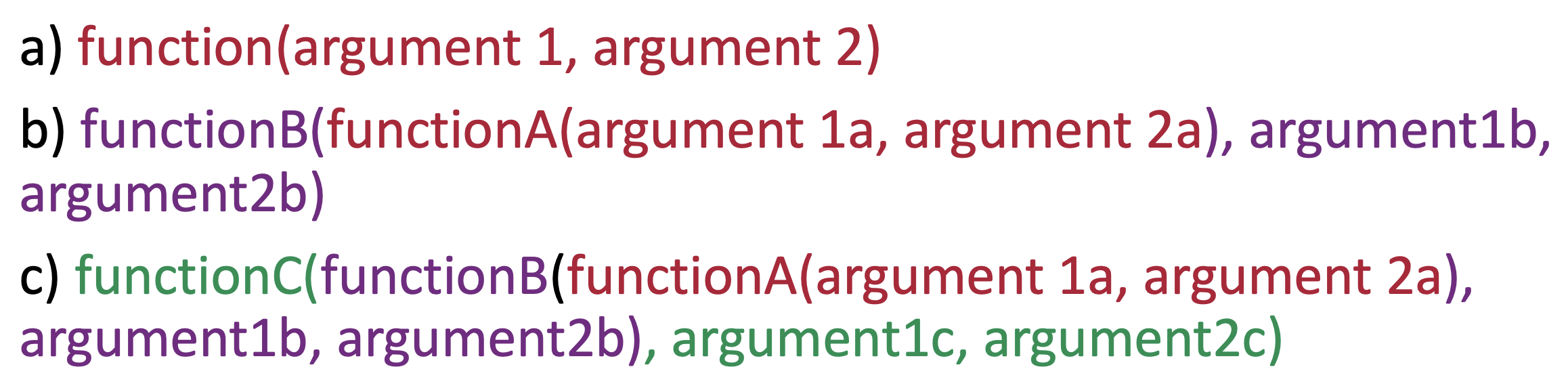
round(mean(L1.Age), digits = 2)

[1] 37.54

In theory, we can nest as many functions as we like, but things can get quite chaotic after more than a couple of functions. We need to make sure that we can trace back which arguments and which brackets belong to which function (see Figure 7.5).

Figure 7.5: A schematic representations of a) one function with two arguments, b) two nested functions each with two arguments, and c) three nested functions each with two arguments

TipTime to think!

Consider the three lines of code below. Without running them, can you tell which of the three lines of code will output the square root of L1 participant’s average age to two decimal places?

round(sqrt(mean(L1.Age) digits = 2))
sqrt(round(mean(L1.Age), digits = 2))
round(sqrt(mean(L1.Age)), digits = 2)

1

This code will return an “unexpected symbol” error because it is missing a comma before the argument digits = 2.

2

This second line of code actually outputs 6.126989, which has more than two decimal places! This is because R interprets the functions from the inside out: first, it calculates the mean value, then it rounds that off to two decimal places, and only then does it compute the square root of that rounded off value.

3

This third attempt, in contrast, does the rounding operation as the last step. Note that, in the two lines of code that do not produce an error, the brackets around the argument digits = 2 are also located in different places.

It is very easy to make bracketing errors when writing code and especially so when nesting functions (see Figure 7.5) so watch your commas and brackets (see also Section 5.6)!

7.5.2 Piped Functions

If you found all these brackets overwhelming: fear not! There is a second method for combining functions in R, which is often more convenient and almost always easier to decipher. It involves the pipe operator, which in R is |>.¹

The |> operator passes the output of one function on to the first argument of the next function. This allows us to chain multiple functions together in a much more intuitive way, e.g.:

L1.Age |> 
 mean() |> 
 round()

[1] 38

In the example above, the object L1.Age is passed on to the first argument of the mean() function. This calculates the mean of L1.Age. Next, this result is passed to the round() function, which rounds the mean value to the nearest integer.

To pass additional arguments to any function in the pipeline, we add them within the brackets that belong to that function:

L1.Age |> 
 mean() |> 
 round(digits = 2)

[1] 37.54

Like many of the relational operators we learnt about in Section 5.5, the R pipe is a combination of two symbols, the computer pipe | and the right angle bracket >. Don’t worry if you’re not sure where these two symbols are on your keyboard as RStudio has a handy shortcut for you: (see also Figure 7.6). I strongly recommend that you write this shortcut on a prominent post-it and learn it asap, as you will need it a lot when you are working in R!²

Figure 7.6: Remix of René Magritte’s “La Trahison des images” with the native R pipe and its RStudio shortcut (Le Foll 2025. Zenodo. https://doi.org/10.5281/zenodo.17440405)

TipYour turn!

Q7.18 Using the R pipe operator, calculate the average mean age of the L2 participants and round off this value to two decimal places. What is the result?

Q7.19 Unsurprisingly, in Dąbrowska (2019)‘s study, English L1 participants, on average, scored higher in the English vocabulary test than L2 participants. Calculate the difference between L1 and L2 participants’ mean Vocab test results and round off this means difference to two decimal places.

🐭 Click on the mouse for a hint.

NoteClick here for a detailed answer to Q7.19

They are lots of ways to tackle this in R. Here is a first approach that involves the pipe operator:

(mean(L1.data$Vocab) - mean(L2.data$Vocab)) |> 
  round(digits = 2)

[1] 16.33

Note that this approach requires a set of brackets around the first subtraction operation, otherwise only the second mean value is rounded off to two decimal places. Compare the following lines of code:

mean(L1.data$Vocab) - mean(L2.data$Vocab)

[1] 16.33315

(mean(L1.data$Vocab) - mean(L2.data$Vocab)) |> 
  round(digits = 2)

[1] 16.33

mean(L1.data$Vocab) - round(mean(L2.data$Vocab), digits = 2)

[1] 16.3358

An alternative approach would be to store the difference in means as an R object and, in a second line of code, pass this object to the round() function.

mean.diff.vocab <- mean(L1.data$Vocab) - mean(L2.data$Vocab)

round(mean.diff.vocab, digits = 2)

[1] 16.33

Or, you could combine both approaches like this:

mean.diff.vocab <- mean(L1.data$Vocab) - mean(L2.data$Vocab)
mean.diff.vocab |> 
  round(digits = 2)

[1] 16.33

There is often more than one way to solve problems in R. Choose whichever way you are most comfortable with. As you long as you understand what your code does (see Chapter 15), it doesn’t matter if it’s particularly elegant or efficient.

Check your progress 🌟

Well done! You have successfully completed 0 out of 19 questions in this chapter.

Are you confident that you can…?

• Inspect a data set in R (Section 7.1)
• Recognise different types of variables (Section 7.2)
• Access individual columns and data points in R (Section 7.2.4)–(Section 7.3)
• Use built-in R functions and change function arguments (Section 7.4)
• Combine functions in R using both the nesting and the piping methods (Section 7.5.1)–(Section 7.5.2)

You are now ready to do statistics in R! 💪 In Chapter 8, we begin with descriptive statistics.

Dąbrowska, Ewa. 2019. Experience, aptitude, and individual differences in linguistic attainment: A comparison of native and nonnative speakers. Language Learning 69(S1). 72–100. https://doi.org/10.1111/lang.12323.

---

1. This is the native R pipe operator, which was introduced in May 2021 with R version 4.1.0. As a result, you will not find it in code written in earlier versions of R. Previously, piping required an additional R library, the {magrittr} library. The {magrittr} pipe looks like this: %>%. At first sight, they appear to work is in the same way, but there are some important differences. If you are familiar with the {magrittr} pipe and want to understand how it differs from the native R pipe, I recommend this excellent blog post by Isabella Velásquez: https://ivelasq.rbind.io/blog/understanding-the-r-pipe/.

2. If, in your version of RStudio, this shortcut produces %>% instead of |>, you have probably not activated the native R pipe option in your RStudio global options (see instructions in Section 4.3.1).