library(tidyverse)9 Data wRangling
Chapter overview
In this chapter, you will learn how to:
- Recognise whether a dataset is in tidy data format
- Check the sanity of an imported dataset
- Pre-process data in a reproducible way using tidyverse functions
- Convert character vectors representing categorical data to factors
- Add and replace columns in a table
- Transform several columns of a table at once
- Use {stringr} functions to manipulate text values
- Reshape and combine tables
- Save and export
Robjects in different formats
9.1 Welcome to the tidyverse! 🪐
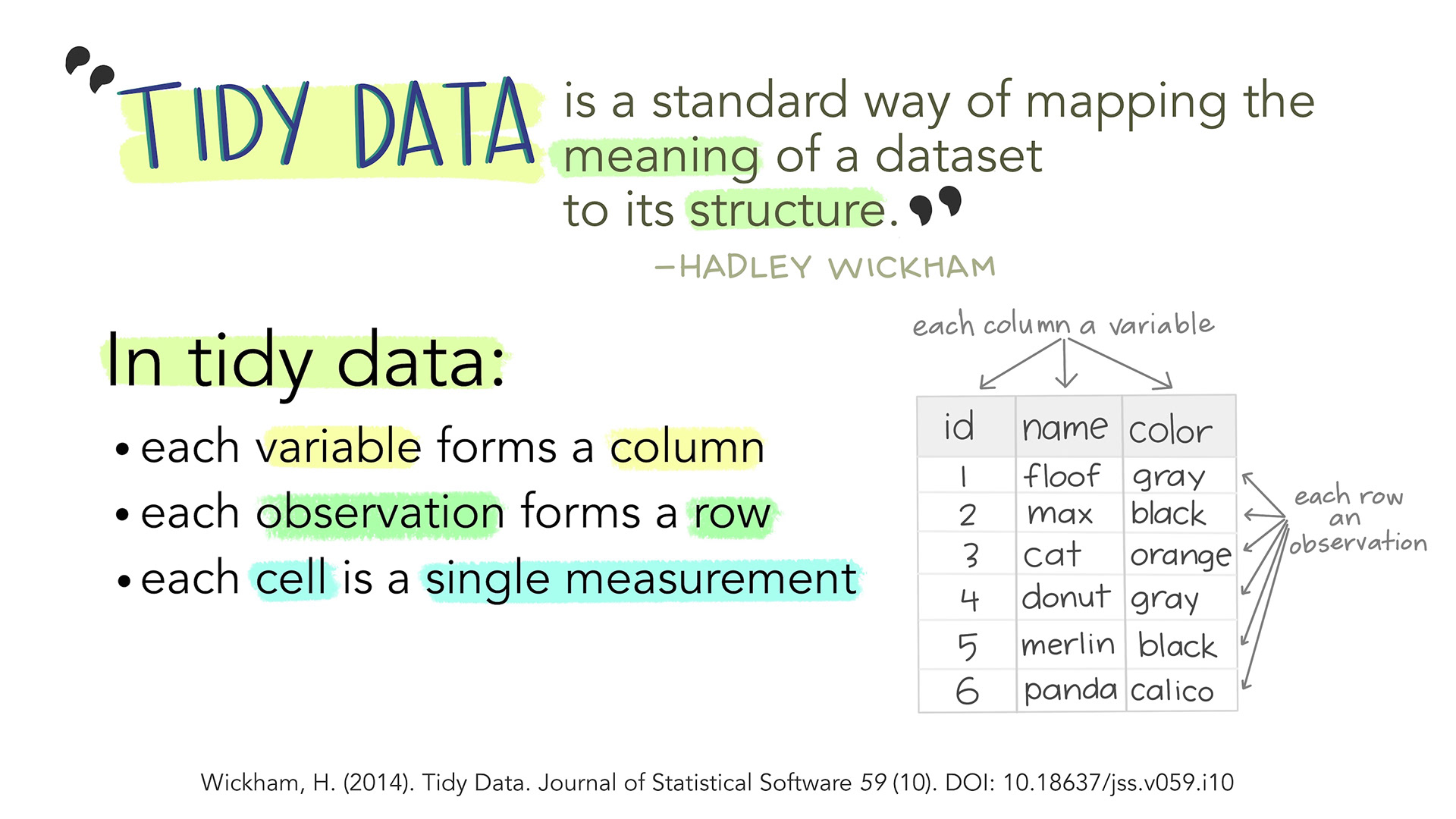
This chapter explains how to examine, clean, and manipulate data mostly using functions from the {tidyverse}: a collection of useful R packages increasingly used for all kinds of data analysis projects. Tidyverse functions are designed to work with tidy data (see Figure 9.1) and, as a result, they are often easier to combine.
Learning to manipulate data and conduct data analysis in R “the tidyverse-way” can help make your workflows more efficient.
If you ensure that your data are tidy, you’ll spend less time fighting with the tools and more time working on your analysis. (Wickham, Vaughan & Girlich 2025)
9.2 Base R vs. tidyverse functions
Novice R users may find it confusing that many operations can be performed using either a base R function or a tidyverse function. For example, in Chapter 6, we saw that both the base R function read.csv() and the tidyverse function read_csv() can be used to import CSV files. The functions have slightly different arguments and default values, which can be annoying, even though they are fundamentally designed to perform the same task. But don’t fret over this too much: it’s fine for you to use whichever function you find most convenient and intuitive and it’s also absolutely fine to combine base R and tidyverse functions!
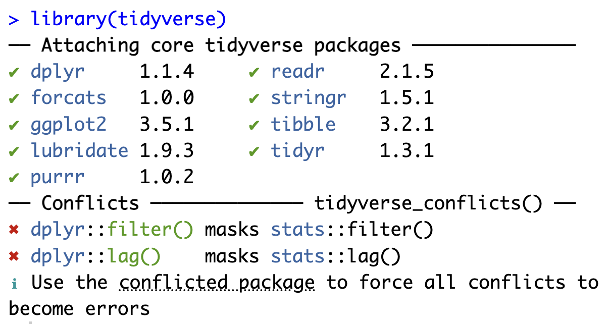
You will no doubt have noticed that the functions read.csv() and read_csv() have very similar but not exactly identical names. This is helpful to differentiate between the two functions. Unfortunately, some function names are found in several packages, which can lead to conflicts and errors! For example, you may have noticed that when you load the tidyverse library the first time in a project, a message similar to Figure 9.2 is printed in the Console (note that you should have more recent installations of these packages).
First, the message reproduced in Figure 9.2 confirms that loading the {tidyverse} library has led to the successful loading of a total of nine packages and that these are now ready to use. Crucially, the message also warns us about conflicts between some {tidyverse} packages and base R packages. These conflicts are due to the fact that two functions from the {dplyr} package have exactly the same name as functions from the base R {stats} package. The warning informs us that, by default, the {dplyr} functions will be applied.
To force R to use a function from a specific package, we can use the package::function() syntax. Hence, to force R to use the base R {stats} filter() function rather than the tidyverse one, we would use stats::filter(). On the contrary, if we want to be absolutely certain that the tidyverse one is used, we can use dplyr::filter().
In this chapter, we will explore functions from {dplyr}, {stringr}, and {tidyr}. The popular {ggplot2} tidyverse library for data visualisation following the Grammar of Graphics approach will be introduced in Chapter 10. Make sure that you have loaded the tidyverse packages before proceeding with the rest of this chapter. If you are encountering package installation issues, head to Section 4.4.2 to fix them before continuing.
9.3 Checking data sanity
Before beginning any data analysis, it is important to always check the sanity of our data. In the following, we will use tables and descriptive statistics to do this. In Chapter 10, we will learn how to use data visualisation to check for outliers and other issues that may affect our statistical analyses.
In this chapter and the following chapters, all examples, tasks, and quiz questions are based on data from Dąbrowska (2019). You will only be able to reproduce the analyses and answer the quiz questions if you have created an RProject and saved the data within the project directory. Detailed instructions to do so can be found from Section 6.3 to Section 6.5.
Alternatively, you can download Dabrowska2019.zip from the textbook’s GitHub repository. To launch the project correctly, first unzip the file and then double-click on the Dabrowska2019.Rproj file.
Before we get started, make sure that both the L1 and the L2 datasets are correctly loaded by checking the structure of the R objects using the str() function.
library(here)

L1.data <- read.csv(file = here("data", "L1_data.csv"))
str(L1.data)

L2.data <- read.csv(file = here("data", "L2_data.csv"))
str(L2.data)
9.3.1 Numeric variables
In Section 8.3.2, we used the summary() function to obtain some useful descriptive statistics on a single numeric variable, namely the range, mean, median, and interquartile range (IQR).
summary(L1.data$GrammarR) Min. 1st Qu. Median Mean 3rd Qu. Max.
58.00 71.25 76.00 74.42 79.00 80.00 To check the sanity of a dataset, we can use this same function on an entire data table (provided that the data are in the tidy format, see Section 9.1). Thus, the command summary(L1.data)1 outputs summary statistics on all the variables of the L1 dataset - in other words, on all the columns of the data frame L1.data.
summary(L1.data) Participant Age Gender Occupation
Length:90 Min. :17.00 Length:90 Length:90
Class :character 1st Qu.:25.00 Class :character Class :character
Mode :character Median :32.00 Mode :character Mode :character
Mean :37.54
3rd Qu.:55.00
Max. :65.00
OccupGroup OtherLgs Education EduYrs
Length:90 Length:90 Length:90 Min. :10.00
Class :character Class :character Class :character 1st Qu.:12.00
Mode :character Mode :character Mode :character Median :13.00
Mean :13.71
3rd Qu.:14.00
Max. :21.00
ReadEng1 ReadEng2 ReadEng3 ReadEng
Min. :0.000 Min. :0.000 Min. :0.000 Min. : 0.000
1st Qu.:1.000 1st Qu.:1.000 1st Qu.:2.000 1st Qu.: 5.000
Median :2.000 Median :2.000 Median :2.000 Median : 7.000
Mean :2.522 Mean :2.433 Mean :2.233 Mean : 7.189
3rd Qu.:3.000 3rd Qu.:3.000 3rd Qu.:3.000 3rd Qu.: 9.750
Max. :5.000 Max. :5.000 Max. :4.000 Max. :14.000 For the numeric variables in the dataset, the summary() function provides us with many useful descriptive statistics to check the sanity of the data. For example, we can check whether the minimum values include improbably low values (e.g. a five-year-old participant in a written language exam) or outright impossible ones (e.g. a minus 18-year old participant!). Equally, if we know that the maximum number of points that could be obtained in the English grammar test is 100, a maximum value of more than 100 would be highly suspicious and warrant further investigation.
As far as we can see from the output of summary(L1.data) above, the numeric variables in Dąbrowska (2019)’s L1 dataset do not appear to feature any obvious problematic values.
9.3.2 Categorical variables as factors
Having examined the numeric variables, we now turn to the non-numeric, categorical ones (see Section 7.2). For these variables, the descriptive statistics returned by summary(L1.data) are not as insightful. They only tell us that they each include 90 values, which corresponds to the 90 participants in the L1 dataset. As we can see from the output of the str() function, these categorical variables are stored in R as character string vectors (abbreviated in the str() output to “chr”).
str(L1.data$Gender) chr [1:90] "M" "M" "M" "F" "F" "F" "F" "M" "M" "F" "F" "M" "M" "F" "M" "F" ...Character string vectors are a useful R object type for text but, in R, categorical variables are best stored as factors. Factors are a more efficient way to store character values because each unique character value is stored only once. The data itself are stored as a vector of integers. Let’s look at an example.
First, we convert the categorical variable Gender from L1.data that is currently stored as a character string vector to a factor vector called L1.Gender.fct:
L1.Gender.fct <- factor(L1.data$Gender)When we now inspect its structure using str(), we can see that L1.Gender.fct is a factor with two levels “F” and “M”. The values themselves, however, are no longer listed as “M” “M” “M” “F” “F”…, but rather as integers: 2 2 2 1 1 1….
str(L1.Gender.fct) Factor w/ 2 levels "F","M": 2 2 2 1 1 1 1 2 2 1 ...By default, the levels of a factor are ordered alphabetically, hence in L1.Gender.fct, 1 corresponds to “F” and 2 to “M”.
The summary output of factor vectors are far more insightful than of character variables (and look rather like the output of the table() function that we used in Section 8.1.3).
summary(L1.Gender.fct) F M
48 42 The tidyverse package {forcats} (Wickham 2025a) has a lot of very useful functions to manipulate factors. They all start with fct_.
Q9.1 Type ?fct_ in an R script or directly in the Console and then press the tab key ( on your keyboard). A list of all loaded functions that start with fct_ should pop up. Which of these is not listed?
Q9.2 In the factor object L1.Gender.fct (which we created above), the first level is “F” because it comes first in the alphabet. Which of these commands will make “M” the first level instead? Check out the help files of the following {forcats} functions to understand what they do and try them out.
9.4 Pre-processing data
9.4.1 Using mutate() to add and replace columns
In the previous section, we stored the factor representing L1 participants’ gender as a separate R object called L1.Gender.fct. If, instead, we want to add this factor as an additional column to our dataset, we can use the mutate() function from {dplyr}.
L1.data <- L1.data |>
  mutate(Gender.fct = factor(L1.data$Gender))
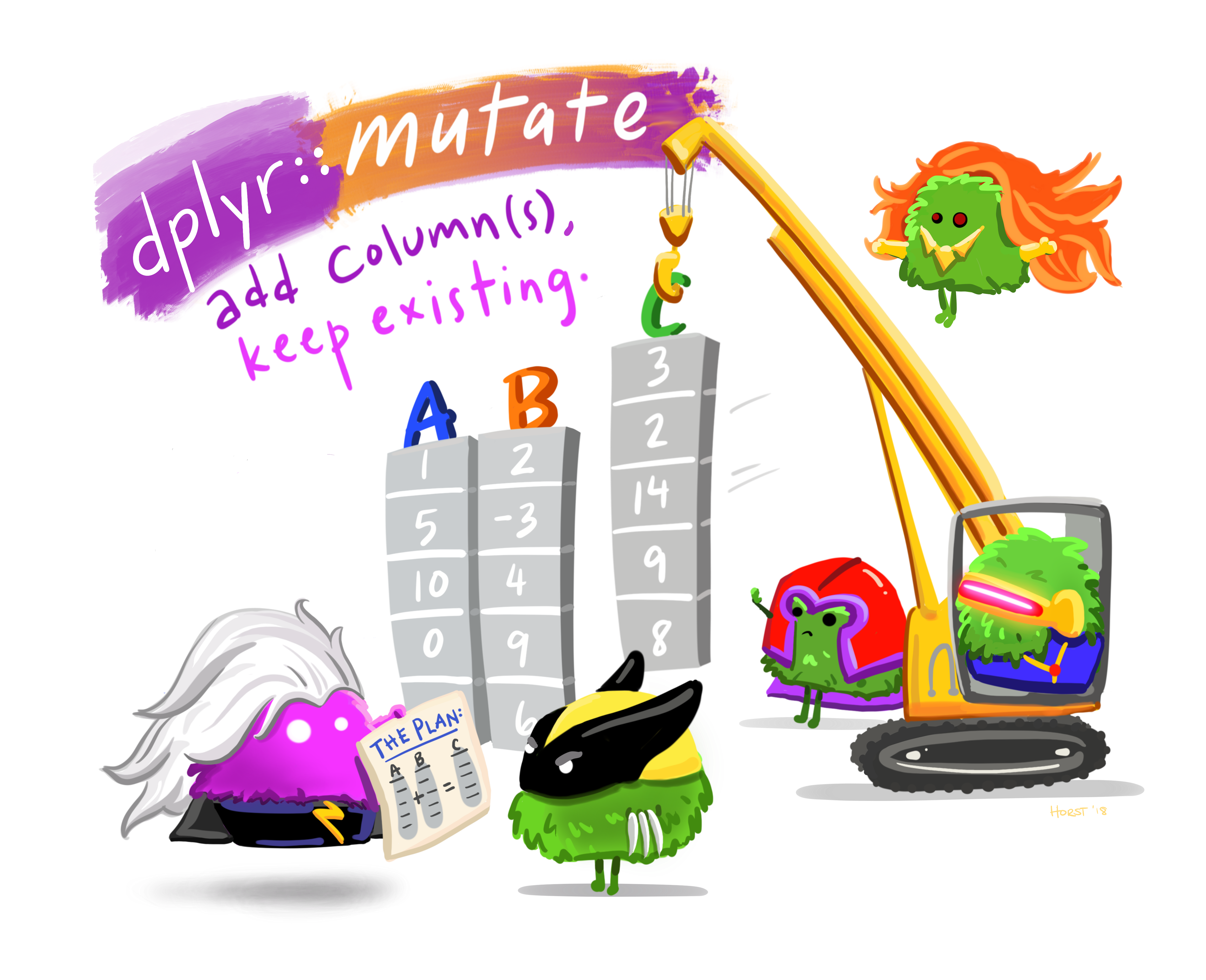
The mutate() function allows us to add new columns to a dataset (see Figure 9.3). By default, it also keeps all the existing ones. To control which columns are retained, check the help file and read about the .keep argument.
dplyr::mutate() function CC BY 4.0 @allison_horst.
We can use the colnames() function to check that the new column has been correctly appended to the table. Alternatively, you can use the View() function to display the table in full in a new RStudio tab. In both cases, you should see that the new column is now the last column in the table (column number 32).
colnames(L1.data) [1] "Participant" "Age" "Gender" "Occupation" "OccupGroup"
[6] "OtherLgs" "Education" "EduYrs" "ReadEng1" "ReadEng2"
[11] "ReadEng3" "ReadEng" "Active" "ObjCl" "ObjRel"
[16] "Passive" "Postmod" "Q.has" "Q.is" "Locative"
[21] "SubCl" "SubRel" "GrammarR" "Grammar" "VocabR"
[26] "Vocab" "CollocR" "Colloc" "Blocks" "ART"
[31] "LgAnalysis" "Gender.fct" Watch out: if you add a new column to a table using an existing column name, mutate() will overwrite the entire content of the existing column with the new values! In the following code chunk, we are therefore overwriting the character vector Gender with a factor vector also called Gender. We should only do this if we are certain that we won’t need to compare the original values with the new ones!
L1.data <- L1.data |>
  mutate(Gender = factor(L1.data$Gender))
9.4.2 Using across() to transform multiple columns
In addition to Gender, there are quite a few more character vectors in L1.data that represent categorical variables and that would therefore be better stored as factors. We could use mutate() and factor() to convert them one by one like we did for Gender above, but that would require several lines of code in which we could easily make a silly error or two. Instead, we can use a series of neat tidyverse functions to convert all character vectors to factor vectors in one go.
L1.data.fct <- L1.data |>
  mutate(across(where(is.character), factor))
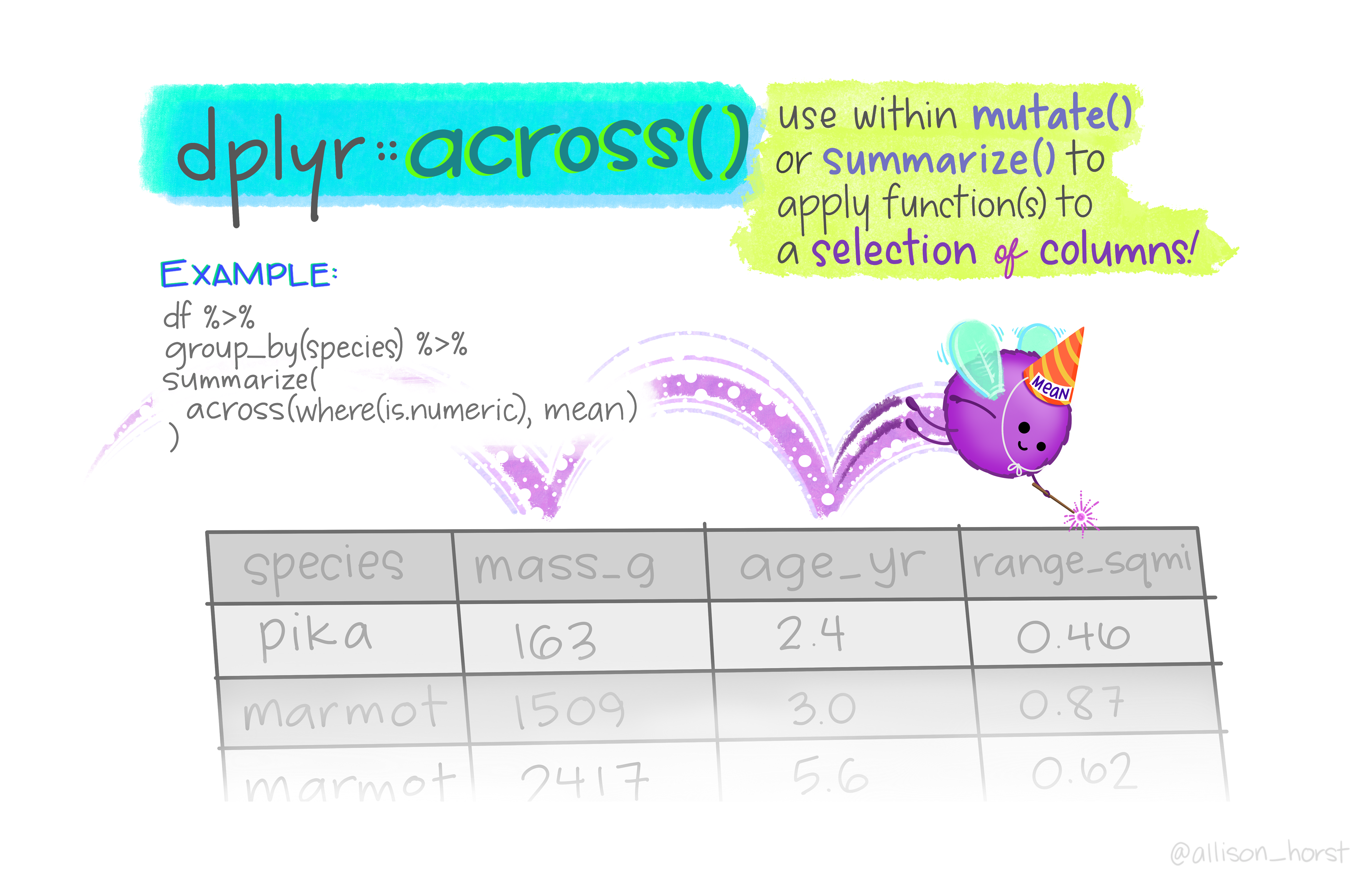
Above, we use mutate() to convert across() the entire dataset all columns where() there are character vectors to factor() vectors (using the is.character() function to determine which columns contain character vectors).
across() function CC BY 4.0 @allison_horst.
We can check that the correct variables have been converted by comparing the output of summary(L1.data) (partially printed in Section 9.3.1) with the output of summary(L1.data.fct) (partially printed below).
summary(L1.data.fct) Participant Age Gender Occupation OccupGroup
1 : 1 Min. :17.00 F:48 Retired :14 C :22
100 : 1 1st Qu.:25.00 M:42 Student :14 I :23
101 : 1 Median :32.00 Unemployed : 4 M :20
104 : 1 Mean :37.54 Housewife : 3 PS :24
106 : 1 3rd Qu.:55.00 Shop Assistant: 3 PS : 1
107 : 1 Max. :65.00 Teacher : 3
(Other):84 (Other) :49
OtherLgs Education EduYrs
French : 2 student : 8 Min. :10.00
German : 3 A level : 5 1st Qu.:12.00
None :84 BA : 5 Median :13.00
Spanish: 1 GCSEs : 5 Mean :13.71
NVQ : 4 3rd Qu.:14.00
Northern Counties School Leaving Exam: 3 Max. :21.00
(Other) :60
ReadEng1 ReadEng2 ReadEng3 ReadEng
Min. :0.000 Min. :0.000 Min. :0.000 Min. : 0.000
1st Qu.:1.000 1st Qu.:1.000 1st Qu.:2.000 1st Qu.: 5.000
Median :2.000 Median :2.000 Median :2.000 Median : 7.000
Mean :2.522 Mean :2.433 Mean :2.233 Mean : 7.189
3rd Qu.:3.000 3rd Qu.:3.000 3rd Qu.:3.000 3rd Qu.: 9.750
Max. :5.000 Max. :5.000 Max. :4.000 Max. :14.000
In this task, you will do some data wrangling on the L2 dataset from Dąbrowska (2019).
Q9.3 Which of these columns from L2.data represent categorical variables and therefore ought to be converted to factors?
Q9.4 Convert all character vectors of L2.data to factors and save the new table as L2.data.fct. Use the str() function to check that your conversion has worked as planned. How many different factor levels are there in the categorical variable Occupation?
Click here to view R code to help you answer c.
L2.data.fct <- L2.data |>
  mutate(across(where(is.character), factor))

str(L2.data.fct)
Q9.5 Use the summary() and str() functions to inspect the sanity of L2 dataset now that you have converted all the character vectors to factors. Have you noticed that there are three factor levels in the Gender variable of the L2 dataset whereas there are only two in the L1 dataset? What is the most likely reason for this?
9.5 Data cleaning 🧼
By closely examining the data, we noticed that the values of the categorical variables were not always consistent, which may lead to incorrect analyses. For example, in the L2 dataset, most female participants’ gender is recorded as F except for six participants, where it is f. As R is a case-sensitive language, these two factor levels are treated as two different levels of the Gender variable. This means that any future analyses on the effect of Gender on language learning will compare participants across these three groups:
summary(L2.data.fct$Gender) f F M
6 40 21 To ensure that our analyses are reproducible (see Section 14.2) from the raw data to the final statistics and figures, it is crucial that we document all of our corrections and other pre-processing steps in scripts. This ensures that, if we need to go back on any data pre-processing decision that we made or if we need to make any additional corrections, we can do so without having to re-do our entire analyses. For example, what if we later found out that a research assistant had coded participants who failed to provide a gender as f? It would be important to be able to go back to our decision of converting all f entries to F! In addition, coding and documenting our pre-processing steps means that all our analytical decisions are transparent and can be inspected and challenged by our peers.
9.5.1 Using {stringr} functions 🎻
To convert all of the lower-case f in the Gender variable to upper-case F, we can combine the mutate() with the str_to_upper() function. This ensures that all values in the new Gender.corrected column are in capital letters.
L2.data.cleaned <- L2.data.fct |>
  mutate(Gender.corrected = str_to_upper(Gender))
We should check that our correction has gone to plan by comparing the original Gender variable with the new Gender.corrected. To this end, we display them side by side using the select() function from {dplyr}.
L2.data.cleaned |>
  select(Gender, Gender.corrected)
Gender Gender.corrected
1 F F
2 f F
3 F F
4 F F
5 M M
6 F FLike mutate() and select(), str_to_upper() also comes from a tidyverse package.2 All functions that begin with str_ come from the {stringr} package (Wickham 2025b), which features lots of useful functions to manipulate character string vectors. These include:
str_to_upper()converts all characters to upper case.str_to_lower()converts all characters to lower case.str_to_title()converts character string title case (i.e. only the first letter of each word is capitalised).str_to_sentence()converts character string to sentence case (i.e. only the first letter of each sentence is capitalised).
For more useful functions to manipulate character strings, check out the {stringr} cheatsheet.
Note that in the code chunk above, we did not save the output to a new R object. We merely printed the output in the Console. Once we have checked that our data wrangling operation went as planned, we can overwrite the original Gender variable with the cleaned version by using the original variable name as the name of the new column. This is no problem because we are not overwriting any data in the original L1_data.csv file, but rather within our R object that we can recreate any time by simply rerunning our script.
L2.data.cleaned <- L2.data.fct |>
  mutate(Gender = str_to_upper(Gender))
Using summary() or class(), we can see that manipulating the Gender variable with a function from {stringr} has resulted in the factor variable being converted back to a character variable.
summary(L2.data.cleaned$Gender) Length Class Mode
67 character character class(L2.data.cleaned$Gender)[1] "character"We therefore need to add a line of code to reconvert it to a factor. We can perform both operations within a single mutate() command.
L2.data.cleaned <- L2.data.fct |>
  mutate(Gender = str_to_upper(Gender),
         Gender = factor(Gender))

class(L2.data.cleaned$Gender)
[1] "factor"Now the summary() function provides a tally of male and female participants that corresponds to the values reported in Dąbrowska (2019: 5).
summary(L2.data.cleaned$Gender) F M
46 21 This task focuses on the OccupGroup variable, which is found in both the L1 and L2 datasets.
OccupGroup is a categorical variable that groups participants’ professional occupations into different categories. In the L2 dataset, there are four occupational categories.
L2.data.fct |>
  count(OccupGroup)
OccupGroup n
1 C 10
2 I 3
3 M 21
4 PS 33Dąbrowska (2019: 6) explains that these abbreviations correspond to:
C: Clerical positions
I: Occupationally inactive (i.e. unemployed, retired, or homemakers)
M: Manual jobs
PS: Professional-level jobs or studying for a degree
Q9.6 Examine the OccupGroup variable in the L1 dataset (L1.data). What do you notice? Why are L1 participants grouped into five rather than four occupational categories?
Click here for R code to help you Q9.6.
summary(L1.data.fct$OccupGroup)
##   C   I   M  PS PS
##  22  23  20  24   1

L1.data.fct |>
  count(OccupGroup)
##   OccupGroup  n
## 1          C 22
## 2          I 23
## 3          M 20
## 4         PS 24
## 5        PS   1
Q9.7 Which {stringr} function removes trailing spaces from character strings? Find the appropriate function on the {stringr} cheatsheet.
Show R code to use the function and check that it worked as expected.
L1.data.cleaned <- L1.data.fct |>
  mutate(OccupGroup = str_trim(OccupGroup))

L1.data.cleaned |>
  count(OccupGroup)
Q9.8 Following the removal of trailing whitespaces, what percentage of L1 participants have a professional-level jobs/are studying for a degree?
Show R code to help you answer Q9.8.
L1.data.cleaned |>
  count(OccupGroup) |>
  mutate(percent = n / sum(n),
         percent = percent*100,
         percent = round(percent, digits = 2)
         )
So far, we have looked at relatively simple data cleaning processes. Let’s now turn to a slightly more complex one: in the L2 dataset, the variable NativeLg contains character string values that correspond to the L2 participants’ native language. Using the base R function unique(), we can see that there are a total of 22 unique values in this variable. However using sort() to order these 22 values alphabetically, we can easily see that there are, in fact, fewer unique native languages in this dataset due to different spellings and the inconsistent use of upper-case letters:
L2.data$NativeLg |>
  unique() |>
  sort()
[1] "Cantonese" "Cantonese/Hokkein" "chinese"
[4] "Chinese" "french" "German"
[7] "greek" "Italian" "Lithuanian"
[10] "Lithunanina" "Lituanian" "Mandarin"
[13] "Mandarin Chinese" "Mandarin/ Cantonese" "mandarin/malaysian"
[16] "Mandarine Chinese" "polish" "Polish"
[19] "Polish/Russian" "russian" "Russian"
[22] "Spanish" If we convert all NativeLg values to title case, we can reduce the number of unique languages to 19:
L2.data$NativeLg |>
  str_to_title() |>
  unique() |>
  sort()
[1] "Cantonese" "Cantonese/Hokkein" "Chinese"
[4] "French" "German" "Greek"
[7] "Italian" "Lithuanian" "Lithunanina"
[10] "Lituanian" "Mandarin" "Mandarin Chinese"
[13] "Mandarin/ Cantonese" "Mandarin/Malaysian" "Mandarine Chinese"
[16] "Polish" "Polish/Russian" "Russian"
[19] "Spanish" Second, to facilitate further analyses, we may decide to only retain the first word/language from each entry as this will further reduce the number of different levels in this categorical variable. To abbreviate “Mandarin Chinese” to “Mandarin”, we can use the word() function from the {stringr} package.
Below is an extract of the help page for the word() function (accessed with the command ?word). Can you work out how to extract the first word of a character string?
word {stringr} R Documentation Extract words from a sentence
Description
Extract words from a sentence ### Usage {.unnumbered .unlisted}
word(string, start = 1L, end = start, sep = fixed(" "))Arguments
stringInput vector. Either a character vector, or something coercible to one.
start,endPair of integer vectors giving range of words (inclusive) to extract. If negative, counts backwards from the last word.
The default value select the first word.
sepSeparator between words. Defaults to single space.
The help file tells us that “The default value select[s] the first word”. In our case, this means that we can use the word() function with no specified argument as this will automatically retain only the first word of every entry.
L2.data$NativeLg |>
  str_to_title() |>
  word() |>
  unique() |>
  sort()
[1] "Cantonese" "Cantonese/Hokkein" "Chinese"
[4] "French" "German" "Greek"
[7] "Italian" "Lithuanian" "Lithunanina"
[10] "Lituanian" "Mandarin" "Mandarin/"
[13] "Mandarin/Malaysian" "Mandarine" "Polish"
[16] "Polish/Russian" "Russian" "Spanish" Alternatively, we can choose to specify the start argument as a reminder of what we did and to better document our code. The output is exactly the same:
L2.data$NativeLg |>
  str_to_title() |>
  word(start = 1) |>
  unique() |>
  sort()
[1] "Cantonese" "Cantonese/Hokkein" "Chinese"
[4] "French" "German" "Greek"
[7] "Italian" "Lithuanian" "Lithunanina"
[10] "Lituanian" "Mandarin" "Mandarin/"
[13] "Mandarin/Malaysian" "Mandarine" "Polish"
[16] "Polish/Russian" "Russian" "Spanish" As you can tell from the output above, the word() function uses white space to identify word boundaries. In this dataset, however, some of the participants’ native languages are separated by forward slashes (/) rather than or in addition to spaces. The “Usage” section of the help file for the word() function (see ?word and above) also confirms that the default word separator symbol is a space and shows us the syntax for changing the default separator. Below we change it to a forward slash.
L2.data$NativeLg |>
  str_to_title() |>
  word(start = 1, sep = fixed("/")) |>
  unique() |>
  sort()
[1] "Cantonese" "Chinese" "French"
[4] "German" "Greek" "Italian"
[7] "Lithuanian" "Lithunanina" "Lituanian"
[10] "Mandarin" "Mandarin Chinese" "Mandarine Chinese"
[13] "Polish" "Russian" "Spanish" Now we can combine these two word extraction methods using the pipe operator (|>) so that “Cantonese/Hokkein” is abbreviated to “Cantonese” and “Mandarin/ Cantonese” to “Mandarin”.
L2.data$NativeLg |>
str_to_title() |>
word(start = 1) |>
word(start = 1, sep = fixed("/")) |>
unique() |>
sort()- 1
- We first extract the first word before the first space, if any.
- 2
- We then extract the first word before the first forward slash, if any.
 [1] "Cantonese"   "Chinese"     "French"      "German"      "Greek"
 [6] "Italian"     "Lithuanian"  "Lithunanina" "Lituanian"   "Mandarin"
[11] "Mandarine" "Polish" "Russian" "Spanish" Many functions of the {stringr} package involve regular expressions (short: regex). The second page of the {stringr} cheatsheet provides a nice overview of how regular expressions can be used to manipulate character strings in R.
Using the str_extract() function together with the regex \\w+, it is possible to extract the first word of each NativeLg value with just one line of code:
L2.data$NativeLg |>
  str_to_title() |>
  str_extract("\\w+") |>
  unique() |>
  sort()
[1] "Cantonese" "Chinese" "French" "German" "Greek"
[6] "Italian" "Lithuanian" "Lithunanina" "Lituanian" "Mandarin"
[11] "Mandarine" "Polish" "Russian" "Spanish" Regular expressions provide incredibly powerful and versatile ways to work with text in all kinds of programming languages. When conducting corpus linguistics research, they also allow us to conduct complex corpus queries.
Each programming language/software has a slightly different flavour of regex but the basic principles are the same across all languages/software and are well worth learning. To get started, I highly recommend this beautifully designed interactive regex tutorial for beginners by Aykut Kardaş: https://regexlearn.com/learn/regex101. Have fun! :nerd-face:
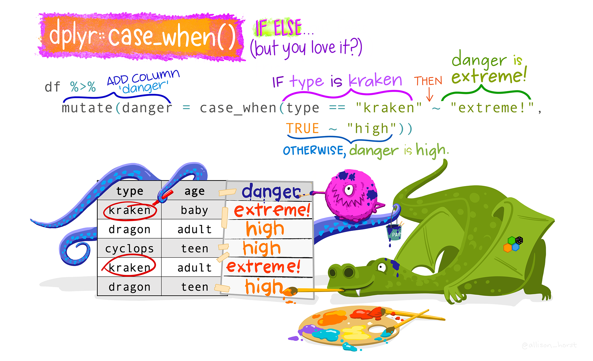
9.5.2 Using case_when()
We have now reduced the number of levels in the NativeLg variable to just 14 unique languages, but we still have some typos to correct, e.g. “Lithunanina” and “Lituanian”. We can correct these on a case-by-case basis using case_when(). This is a very useful tidyverse function from the {dplyr} package that works wonders once we have gotten used to its syntax. Figure 9.5 illustrates the syntax with a toy example dataset about the dangerousness of dragons (df). In this annotated line of code in Figure 9.5, mutate() is used to add a new column called danger whose values depend on the type of dragon that we are dealing with. The first argument of case_when() determines that, when the dragon type is equal to “kraken”, then the danger value is set to “extreme”, otherwise the danger value is set to “high”. You can see the outcome in the danger column.
case_when() function CC BY 4.0 @allison_horst
Applying case_when() to fix the typos in the NativeLg variable in L2.data, we determine that:
- if the shortened
NativeLgvalue is “Mandarine”, we replace it with “Mandarin”, and - if the shortened
NativeLgvalue corresponds to either “Lithunanina” or “Lituanian”, we replace it with “Lithuanian”.
Using mutate(), we save this cleaned-up version of the NativeLg variable as a new column in our L2.data table, which we call NativeLg.cleaned.
L2.data <- L2.data |>
  mutate(
    NativeLg.cleaned = str_to_title(NativeLg) |>
      word(start = 1) |>
      word(start = 1, sep = fixed("/")),
    NativeLg.cleaned = case_when(
      NativeLg.cleaned == "Mandarine" ~ "Mandarin",
      NativeLg.cleaned %in% c("Lithunanina", "Lituanian") ~ "Lithuanian",
      TRUE ~ NativeLg.cleaned)
    )
Whenever we do any data wrangling, it is crucial that we take the time to carefully check that we have not made any mistakes in the process. To this end, we can display the original NativeLg and the new NativeLg.cleaned variables side by side using the select() function:
L2.data |>
  select(NativeLg, NativeLg.cleaned)
NativeLg NativeLg.cleaned
1 Lithuanian Lithuanian
2 polish Polish
3 Polish Polish
4 Italian Italian
5 Lituanian Lithuanian
6 Polish PolishTo save space, only the first six rows of the table are displayed above. Run the code yourself to check the remaining rows.
R functions instead
This chapter focuses on {tidyverse} functions, however all of the above data wrangling and cleaning operations can equally be achieved using base R functions. For example, the mutate() code chunk above could be replaced by the following lines of base R code:
L2.data$NativeLg.cleaned.base <- gsub("([a-zA-Z]+).*", "\\1", L2.data$NativeLg)
L2.data$NativeLg.cleaned.base <- tools::toTitleCase(L2.data$NativeLg.cleaned.base)
L2.data$NativeLg.cleaned.base[L2.data$NativeLg.cleaned.base == "Mandarine"] <- "Mandarin"
L2.data$NativeLg.cleaned.base[L2.data$NativeLg.cleaned.base %in% c("Lithunanina", "Lituanian")] <- "Lithuanian"- 1
-
With the first line, we extract the first string of letters before any space or slash in
NativeLgand save this to a new variable calledNativeLg.cleaned.base. - 2
-
This line converts all the values of the new variable to title case using a base
Rfunction from the {tools} package. The {tools} package comes withRso you don’t need to install it separately but, if you haven’t loaded it earlier in yourRsession, you need to call the function with the prefixtools::so thatRknows where to find thetoTitleCase()function. - 3
- The third line corrects a single typo.
- 4
- This line replaces two typos with a single correction.
If we now compare the variable created with the tidyverse code (NativeLg.cleaned) vs. the one created using base R functions only (NativeLg.cleaned.base), we can see that they are exactly the same.
L2.data |>
  select(NativeLg.cleaned, NativeLg.cleaned.base)
NativeLg.cleaned NativeLg.cleaned.base
1 Lithuanian Lithuanian
2 Polish Polish
3 Polish Polish
4 Italian Italian
5 Lithuanian Lithuanian
6 Polish PolishAn undeniable advantage of sticking to base R functions is that our code is more portable as it does not require the installation of any additional packages, keeping dependencies on external packages to the minimum. However, base R lacks the consistency of the tidyverse framework, which can make certain data transformation tasks considerably more tricky and our code less readable (and therefore less transparent) to ourselves and others.
As we don’t need two versions of the cleaned NativLg variable, we will now remove the NativeLg.cleaned.base column from L2.data. To do so, we use the select() function combined with the - operator to “unselect” the column that we no longer need.
L2.data <- L2.data |>
select(-NativeLg.cleaned.base)For some analyses, it may be useful to group together participants whose native languages come from the same family of languages. For example, French, Spanish and Italian L1 speakers, may be considered as a one group of participants whose native language is a Romance language.
Use mutate() and case_when() to add a new variable to L2.data that corresponds to the L2 participant’s native language family. Call this new variable NativeLgFamily. Use the following language family categories:
- Baltic
- Chinese
- Germanic
- Hellenic
- Romance
- Slavic
If you’re not sure which language family a language belongs to, look it up on Wikipedia (e.g. the Wikipedia page on the German language informs us in a text box at the top of the article that German is a Germanic language).
Q9.9 Which language family is the second most represented among L2 participants’ native languages in Dąbrowska (2019)?
Q9.10 How many L2 participants are native speakers of a language that belongs to the family of Romance languages?
Q9.11 What percentage of L2 participants have a Slavic native language? Round your answer to the nearest percent.
Q9.12 If you check the output of colnames(L2.data) or View(L2.data), you will see that the new variable that you created is now the last column in the table. Consult the help file of the {dplyr} function relocate() to work out how to place this column immediately after NativeLg.
As is often the case, there are several ways to solve these Your turn! tasks. Here is one solution based on what we have covered so far in this chapter.
Q9.9 Note that the following code will only work if you followed the instructions in the section above to create the NativeLg.cleaned variable as it relies on this variable to create the new NativeLgFamily variable.
L2.data <- L2.data |>
  mutate(NativeLgFamily = case_when(
    NativeLg.cleaned == "Lithuanian" ~ "Baltic",
    NativeLg.cleaned %in% c("Cantonese", "Mandarin", "Chinese") ~ "Chinese",
    NativeLg.cleaned == "German" ~ "Germanic",
    NativeLg.cleaned == "Greek" ~ "Hellenic",
    NativeLg.cleaned %in% c("French", "Italian", "Spanish") ~ "Romance",
    NativeLg.cleaned %in% c("Polish", "Russian") ~ "Slavic"))
As always, it is important to check that things have gone to plan.
L2.data |>
  select(NativeLg.cleaned, NativeLgFamily)
NativeLg.cleaned NativeLgFamily
1 Lithuanian Baltic
2 Polish Slavic
3 Polish Slavic
4 Italian Romance
5 Lithuanian Baltic
6 Polish SlavicQ9.10 We can display the distribution of language families using either the base R table() function or the {tidyverse} count() function.
table(L2.data$NativeLgFamily)
  Baltic  Chinese Germanic Hellenic  Romance   Slavic
       5       15        1        1        6       39
L2.data |>
count(NativeLgFamily) NativeLgFamily n
1 Baltic 5
2 Chinese 15
3 Germanic 1
4 Hellenic 1
5 Romance 6
6 Slavic 39Q9.11 We can add a column to show the distribution in percentages by adding a new “percent” column to the count() table using mutate():
L2.data |>
count(NativeLgFamily) |>
mutate(percent = n / sum(n),
percent = percent*100,
percent = round(percent, digits = 0)
) |>
arrange(desc(n))- 1
-
We start with the dataset that contains the new
NativeLgFamilyvariable. - 2
-
We pipe it into the
count()function. As shown above, this function produces a frequency table with counts stored in the variablen. - 3
-
We divide the number of participant with each native language (
n) by the total number of participants (sum(n)). We obtain proportions ranging from 0 to 1. - 4
- We multiply these by 100 to get percentages.
- 5
- We round the percentages to two decimal places.
- 6
-
We reorder the table so that the most represented group is at the top. To do so, we pipe our table into the
dplyr::arrange(). By default,arrange()orders values in ascending order (from smallest to largest); hence, we add thedesc()function to sort the table in descending order of frequency.
  NativeLgFamily  n percent
1         Slavic 39      58
2        Chinese 15      22
3        Romance  6       9
4         Baltic  5       7
5       Germanic  1       1
6       Hellenic  1       1
🪐 Note that this a {tidyverse} approach to working out percentages, see Section 8.1.3 for a base R approach.
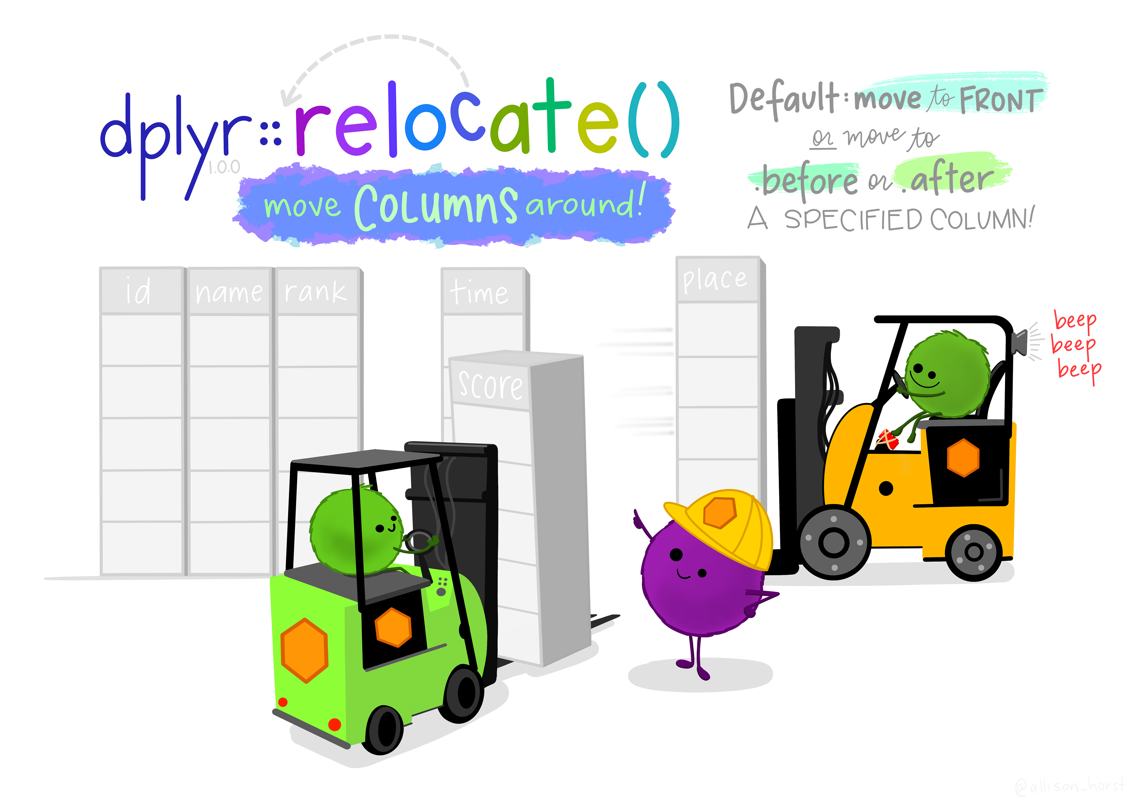
Q9.12 At the time of writing, the help file of the relocate() function still featured examples using the {magrittr} pipe (%>%) rather than the native R pipe (|>) (see Section 7.5.2), but the syntax remains the same. The first argument is the data which we are piping into the function, the second argument is the column that we want to move. Then, we need to specify where to with either the .after or the .before argument.
L2.data <- L2.data |>
relocate(NativeLgFamily, .after = NativeLg)dplyr::relocate() function CC BY 4.0 @allison_horst.
Note that the help file specifies that both “.after” and “.before” begin with a dot. If you leave the dot out, the function will not work as expected! Can you spot what has happened here?
L2.data |>
  relocate(NativeLgFamily, after = NativeLg) |>
  str()
'data.frame': 67 obs. of 6 variables:
$ Participant : int 220 244 46 221 222 230 247 237 243 213 ...
$ Gender : chr "F" "f" "F" "F" ...
$ Occupation : chr "Student" "student" "Cleaner" "Student" ...
$ OccupGroup : chr "PS" "PS" "M" "PS" ...
$ NativeLg : chr "Lithuanian" "polish" "Polish" "Italian" ...
$ NativeLgFamily: chr "Baltic" "Slavic" "Slavic" "Romance" ...The relocate() function has moved NativeLgFamily to the first column (the function’s default position) and has also moved NativeLg to the second position, but it has renamed the column after.
This is a reminder to always check whether your data wrangling operations have gone as planned. Just because you didn’t get an error message doesn’t mean that your code did what you wanted! ⚠️
9.6 Combining datasets
So far, we have analysed the L1 and L2 datasets individually. In the following chapters, however, we will conduct comparative analyses, comparing the performance of the L1 and L2 participants in the various language-related tests conduced as part of Dąbrowska (2019). To this end, we need to create a combined table that includes the data of all participants from Dąbrowska (2019). Recall that both tables, L1.data and L2.data, are in a tidy data format (Figure 9.1). This means that:
- each row represents an observation (i.e. here, a participant),
- each cell represents a measurement, and
- each variable forms a column.
To combine the two datasets, therefore, we need to combine the rows of the two tables. However, we cannot simply add the rows of the L2.data table to the bottom of L1.data table because, as shown below, the two tables do not have the same number of columns and their shared columns are not in the same position!
colnames(L1.data) [1] "Participant" "Age" "Gender" "Occupation" "OccupGroup"
[6] "OtherLgs" "Education" "EduYrs" "ReadEng1" "ReadEng2"
[11] "ReadEng3" "ReadEng" "Active" "ObjCl" "ObjRel"
[16] "Passive" "Postmod" "Q.has" "Q.is" "Locative"
[21] "SubCl" "SubRel" "GrammarR" "Grammar" "VocabR"
[26] "Vocab" "CollocR" "Colloc" "Blocks" "ART"
[31] "LgAnalysis" "Gender.fct" colnames(L2.data) [1] "Participant" "Gender" "Occupation" "OccupGroup"
[5] "NativeLg" "NativeLgFamily" "OtherLgs" "EdNative"
[9] "EdUK" "Age" "EduYrsNat" "EduYrsEng"
[13] "EduTotal" "FirstExp" "Arrival" "LoR"
[17] "EngWork" "EngPrivate" "ReadEng1" "ReadOth1"
[21] "ReadEng2" "ReadOth2" "ReadEng3" "ReadOth3"
[25] "ReadEng" "ReadOth" "Active" "ObjCl"
[29] "ObjRel" "Passive" "Postmod" "Q.has"
[33] "Q.is" "Locative" "SubCl" "SubRel"
[37] "GrammarR" "Grammar" "VocabR" "Vocab"
[41] "CollocR" "Colloc" "Blocks" "ART"
[45] "LgAnalysis" "UseEngC" "NativeLg.cleaned"We therefore need to ensure that, when the two datasets are combined, the shared columns are aligned. Note, also, that participants’ total number of years in education is stored in the EduYrs column in L1.data, whereas the corresponding column in L2.data is called EduTotal. Hence, we first use the {dplyr} function rename() to rename EduYrs in L1.data as EduTotal before we merge the two R objects.
L1.data <- L1.data |>
  rename(EduTotal = EduYrs)
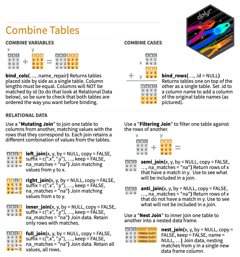
The {dplyr} package boasts a host of useful functions to combine tables (see Figure 9.7). For our purposes, bind_rows() appears to be the perfect function.3
However, when we try to combine L1.data and L2.data using bind_rows(), we get an error message… Does this error remind you of Q7.10 from Chapter 7 by any chance?
combined.data <- bind_rows(L1.data, L2.data)Error in `bind_rows()`:
! Can't combine `..1$Participant` <character> and `..2$Participant` <integer>.What this error message tells us is that the bind_rows() function cannot combine the two Participant columns because, in L1.data, Participant is a string character vector whereas, in L2.data, it is an integer vector. To avoid data loss, bind_rows() can only match columns of the same data type! We must therefore first convert the Participant variable in L2.data to a character vector:
L2.data <- L2.data |>
  mutate(Participant = as.character(Participant))
Having done this, we can use bind_rows() to combine the two tables:
combined.data <- bind_rows(L1.data, L2.data)The problem is that now that we have merged our two datasets into one, it’s not obvious which rows correspond to L1 participants and which to L2 participants! There are various ways to solve this, but here’s a simple three-step solution that relies exclusively on functions that you are already familiar with.
Step 1: We add a new column to L1.data called Group and fill this column with the value “L1” for all rows.
L1.data <- L1.data |>
  mutate(Group = "L1")
Step 2: We add a new column to L2.data also called Group and fill this column with the value “L2” for all rows.
L2.data <- L2.data |>
  mutate(Group = "L2")
Step 3: We use bind_rows() to combine the two datasets that now each include the extra Group column.4
combined.data <- bind_rows(L1.data, L2.data)Verification step: The combined.data table now includes the column Group, which we can use to easily identify the observations that belong to L1 and L2 participants. As expected, our combined dataset includes 90 participants from the L1 group and 67 from the L2 group:
combined.data |>
  count(Group)
Group n
1 L1 90
2 L2 67Our combined dataset contains all the columns that appear in either L1.data or L2.data. Check that this is the case by examining the structure of the new dataset with str(combined.data).
You should have noticed that, in some columns, there are lots of NA (“Not Available”) values. These represent missing data. R has inserted these NA values in the columns that only appear in one of the two datasets. For example, the L1 dataset does not include an Arrival variable (indicating the age when participants first arrived in an English-speaking country), presumably because they were all born in an English-speaking country. We only have this information for the L2 participants and this explains the 90 NA values in the Arrival column of the combined dataset.
combined.data$Arrival [1] NA NA NA NA NA NA NA NA NA NA NA NA NA NA NA NA NA NA NA NA NA NA NA NA NA
[26] NA NA NA NA NA NA NA NA NA NA NA NA NA NA NA NA NA NA NA NA NA NA NA NA NA
[51] NA NA NA NA NA NA NA NA NA NA NA NA NA NA NA NA NA NA NA NA NA NA NA NA NA
[76] NA NA NA NA NA NA NA NA NA NA NA NA NA NA NA 17 18 19 19 19 19 20 22 22 23
[101] 24 25 26 26 28 28 30 44 45 49 17 23 23 24 19 22 23 26 16 18 24 24 25 29 30
[126] 32 33 22 25 30 44 27 18 20 21 33 38 47 16 19 20 24 25 28 33 20 22 25 28 26
[151] 26 16 24 32 20 16 20We can also check this by cross-tabulating the Group and the Arrival variables.
combined.data |>
  count(Group, Arrival)
Group Arrival n
1 L1 NA 90
2 L2 16 4
3 L2 17 2
4 L2 18 3
5 L2 19 6
6 L2 20 6Run View(combined.data) to inspect the combined dataset and check in which other columns there are NA values.
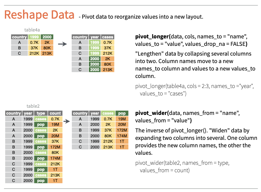
Combining the two datasets from Dąbrowska (2019) was relatively easy because the data was already in tidy format. But, fear not: if you need to first convert your data to tidy format, the {tidyr} package has got you covered!
The pivot_longer() and pivot_wider() functions allow you to easily convert tables from “long” to “wide” format and vice versa (see Figure 9.8).
Remember to carefully check the output of any data manipulation that you do before moving on to doing any analyses! To this end, the str() and View() functions are particularly helpful.
Note that older textbooks/tutorials and AI products such as ChatGPT, Claude, and CoPilot that have been trained on older web data will frequently suggest superseded (i.e. outdated) functions for data manipulation such as spread(), gather(), select_all(), and mutate_if(). If you use superseded functions, your code will still work, but R will print a warning in the Console and usually suggest a more modern alternative.
AI products may also suggest using functions that are deprecated. As with superseded functions, you will get a warning message with a recommended alternative. In this case, however, you must follow the advice of the warning, as writing new code with deprecated functions is really asking for trouble! Deprecated functions are scheduled for removal, which means that your code will eventually no longer run on up-to-date R versions.
In sum, to ensure the future compatibility of your code, do not ignore warnings about deprecated functions and, in general, never ever blindly trust the output of AI tools! More on the use of AI for research and learning in Chapter 15.
9.7 A pre-processing pipeline
So far in this chapter, we have learnt how to pre-process data for future statistical analyses and data visualisation. In the process, we have learnt about lots of different functions, mostly from the tidyverse environment (see Section 9.1 🪐). Now it’s time to put everything together and save our pre-processed combined dataset for future use.
But, first, let’s recap all of the data wrangling operations that we performed in this chapter and combine them into one code chunk. Before running this code, we first reload the original data from Dąbrowska (2019) to overwrite any changes that were made during this chapter. This will ensure that we all have exactly the same version of the dataset for the following chapters. Detailed instructions to download and load the original data can be found in Chapter 6.
library(here)

L1.data <- read.csv(file = here("data", "L1_data.csv"))
L2.data <- read.csv(file = here("data", "L2_data.csv"))
Then, copy and run the following lines of code to create a new R object called combined.data that contains the wrangled data.
If you hover your mouse over the top-right corner of any code chunk in the online version of this textbook, a clipboard symbol will appear. Clicking on this symbol will copy the entire chunk. You can then paste the code in your R script using the shortcut .
L2.data <- L2.data |>
  mutate(Participant = as.character(Participant)) |>
  mutate(Group = "L2")

L1.data <- L1.data |>
  mutate(Group = "L1") |>
  rename(EduTotal = EduYrs)

combined.data <- bind_rows(L1.data, L2.data) |>
  mutate(across(where(is.character), str_to_title)) |>
  mutate(across(where(is.character), str_trim)) |>
  mutate(OccupGroup = str_to_upper(OccupGroup)) |>
  mutate(
    NativeLg = word(NativeLg, start = 1),
    NativeLg = word(NativeLg, start = 1, sep = fixed("/")),
    NativeLg = case_when(
      NativeLg == "Mandarine" ~ "Mandarin",
      NativeLg %in% c("Lithunanina", "Lithunanina", "Lituanian") ~ "Lithuanian",
      TRUE ~ NativeLg)) |>
  mutate(NativeLgFamily = case_when(
    NativeLg == "Lithuanian" ~ "Baltic",
    NativeLg %in% c("Cantonese", "Mandarin", "Chinese") ~ "Chinese",
    NativeLg == "German" ~ "Germanic",
    NativeLg == "Greek" ~ "Hellenic",
    NativeLg %in% c("French", "Italian", "Spanish") ~ "Romance",
    NativeLg %in% c("Polish", "Russian") ~ "Slavic")) |>
  mutate(across(where(is.character), factor))
Don’t forgot to check the result by examining the output of View(combined.data) and str(combined.data).
summary(combined.data) Participant Age Gender Occupation OccupGroup
1 : 1 Min. :17.00 F:94 Student :27 C :32
100 : 1 1st Qu.:25.00 M:63 Retired :15 I :26
101 : 1 Median :31.00 Product Operative: 5 M :41
104 : 1 Mean :35.48 Teacher : 5 PS:58
106 : 1 3rd Qu.:42.00 Cleaner : 4
107 : 1 Max. :65.00 Unemployed : 4
(Other):151 (Other) :97
OtherLgs Education EduTotal ReadEng1
None :98 Student: 8 Min. : 8.50 Min. :0.000
No :11 A Level: 5 1st Qu.:13.00 1st Qu.:1.000
English : 8 Ba : 5 Median :14.00 Median :3.000
German : 6 Gcses : 5 Mean :14.62 Mean :2.599
English At School: 3 Nvq : 4 3rd Qu.:17.00 3rd Qu.:4.000
English, German : 2 (Other):63 Max. :24.00 Max. :5.000
(Other) :29 NA's :67
ReadEng2 ReadEng3 ReadEng
Min. :0.000 Min. :0.000 Min. : 0.000
1st Qu.:1.000 1st Qu.:1.000 1st Qu.: 5.000
Median :2.000 Median :2.000 Median : 7.000
Mean :2.465 Mean :2.019 Mean : 7.083
3rd Qu.:3.000 3rd Qu.:3.000 3rd Qu.:10.000
Max. :5.000 Max. :4.000 Max. :14.000
Q9.13 The following operations describe the steps performed by the data wrangling code chunk above. In which order are the operations performed?
Q9.14 In the combined dataset, how many participants have a clerical occupation?
Q9.15 Of the participants who have a clerical occupation, how many were over 50 years old at the time of the data collection?
R code to answer Q9.15
There are various ways to find the answer to Q5. Sticking to a function that we have looked at so far, you could cross-tabulate Age and OccupGroup using the count() function.
combined.data |>
  count(OccupGroup, Age)
OccupGroup Age n
1 C 20 1
2 C 25 6
3 C 27 2
4 C 28 3
5 C 29 4
6 C 30 3
7 C 32 3
8 C 37 1
9 C 38 1
10 C 39 1
11 C 41 1
12 C 51 2
13 C 52 1
14 C 53 1
15 C 57 1
16 C 60 1And then add up the frequencies listed in the rows that correspond to participants with clerical jobs who are 50.
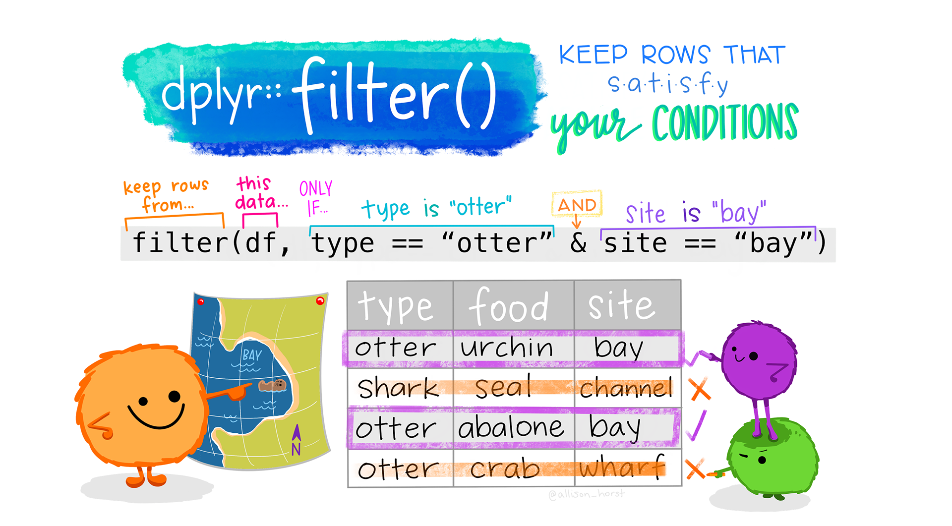
2 + 1 + 1 + 1 +1 [1] 6But, of course, this is method is rather error-prone! Instead, we can use dplyr::filter() (see below) to filter the combined dataset according to our two criteria of interest and then count the number of rows (i.e. participants) remaining in the dataset once the filter has been applied.
combined.data |>
  filter(OccupGroup == "C" & Age > 50) |>
  nrow()
[1] 6dplyr::filter() function CC BY 4.0 @allison_horst.9.8 Saving and exporting R objects 💾
As a final step, we want to save the R object combined.data to a local file on our computer so that, when we continue our analyses in a new R session, we can immediately start working with the wrangled dataset. We can either save the wrangled dataset as an R object (.rds) or export it as a DSV file (e.g. .csv, see Section 2.5.1). The pros and cons of these two solutions are summarised in Table 9.1.
R data files
DSV files (e.g. .csv, .tsv, .tab) |
R data files (.rds) |
|---|---|
| ✅ Highly portable (i.e., can be opened in all standard spreadsheet software and text editors). | ❌ Specific to R and cannot be opened in standard spreadsheet software or text editors. |
| ❌ Inefficient for very large datasets. | ✅ Efficient memory usage for more compact data storage and faster loading times in R. |
| ✅ Universal, language-independent format and therefore suitable for long-term archiving. | ❌ No guarantee that older .rds files will be compatible with newer versions of R and therefore unsuitable for long-term archiving. |
| ❌ Loss of metadata. | ✅ Preserve R data structures (e.g., factor variables remain stored as factors). |
We save both a .csv and an .rds version of the wrangled data. We save both files to a subfolder of our project “data” folder called “processed” using the {here} package to manage the file path (see Section 6.5). If we try to save the file to this subfolder before it has been created at this location we get an error message.
saveRDS(combined.data, file = here("data", "processed", "combined_L1_L2_data.rds"))Error in gzfile(file, mode) : cannot open the connectionWe first need to create the “processed” subfolder before we can save to this location! There are two ways of doing this. In the Files pane of RStudio or in a File Navigator/Explorer window, we can navigate to the “data” folder and, from there, click on the “Create a new folder” icon to create a new subfolder called “processed”.
Alternatively, we can use the dir.create() function to create the subfolder from R itself. If the folder already exists at this location, we will get a warning.
dir.create(file.path(here("data", "processed")))Now that the subfolder exists, we can save combined.data as an .rds file. We will work with this file in the following chapters.
saveRDS(combined.data, file = here("data", "processed", "combined_L1_L2_data.rds"))If you want to share your wrangled dataset with a colleague who does not (yet? 😉) use R, you can use the tidyverse function write_csv().5 Your colleague will be able to open this file in any standard spreadsheet programme or text editor (but do warn them about the dangers of opening .csv file in spreadsheets, see Section 2.6!).
write_csv(combined.data, file = here("data", "processed", "combined_L1_L2_data.csv"))Check your progress 🌟
You have successfully completed 0 out of 15 questions in this chapter.
Are you confident that you can…?
That was a lot of data wrangling, but we are now ready to proceed with some comparative analyses of L1 and L2 English speakers’ language skills! In Chapter 10 we continue to explore the tidyverse as we learn how to use the popular tidyverse package {ggplot2} to visualise the pre-processed data from Dąbrowska (2019). Are you ready to get creative? 🎨
Note that, throughout this chapter, long code output is shortened to save space. When you run this command on your own computer, however, you will see that the output is much longer than what is reprinted in this chapter. You will likely need to scroll up in your Console window to view it all.↩︎
The equivalent base
Rfunction istoupper().↩︎We could also use the
full_join()function since we want to retain all rows and all columns from both datasets.↩︎Alternatively, you may have gathered from the {dplyr} cheatsheet (Figure 9.7) that the
bind_rows()function has an optional.idargument that can be used to create an additional column to disambiguate between the two combined datasets. In this case, we do not need to add aGroupcolumn to both datasets prior to combining them.↩︎combined.data <- bind_rows(L1 = L1.data, L2 = L2.data, .id = "Group")As usual, there is a base
Ralternative:write.csv()will work just as well but, for very large datasets, it is slower thanwrite_csv(). For finer differences, check out the functions’ respective help files.↩︎
