🐭 Click on the mouse for a hint.
14 RepRoducible research and academic wRiting in Quarto
Chapter overview
So far, we have seen how we can export the outputs of our analyses conducted in R in the form of tables (Section 9.8) and graphics (Section 10.3). However, in most situations, we want to communicate our research in a way that allows us to combine both text and analysis outputs. This is where literate programming comes into play!
In this chapter, you will learn:
- about the concept of literate programming
- why reproducibility matters
- how to make your research more reproducible
- how to use Quarto to write research reports, theses, and academic papers
- how to export and share your research in different formats including HTML, PDF, LibreOffice Writer, and Microsoft Word.
Note that a standalone version of this chapter can be found at https://elenlefoll.quarto.pub/quarto4research.
14.1 Literate programming
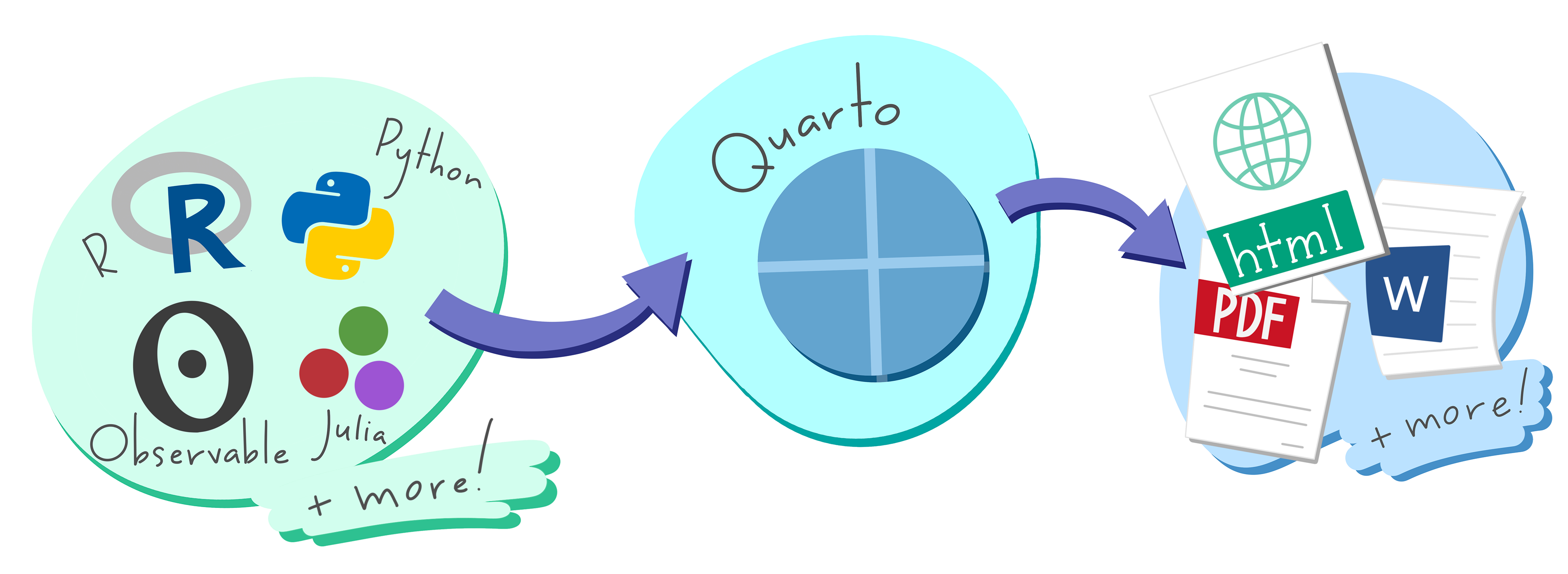
The basic idea of literate programming is that we combine text, code, and code outputs (i.e. tables, statistics, and plots) within a single document that can be exported into different formats for sharing and publishing.
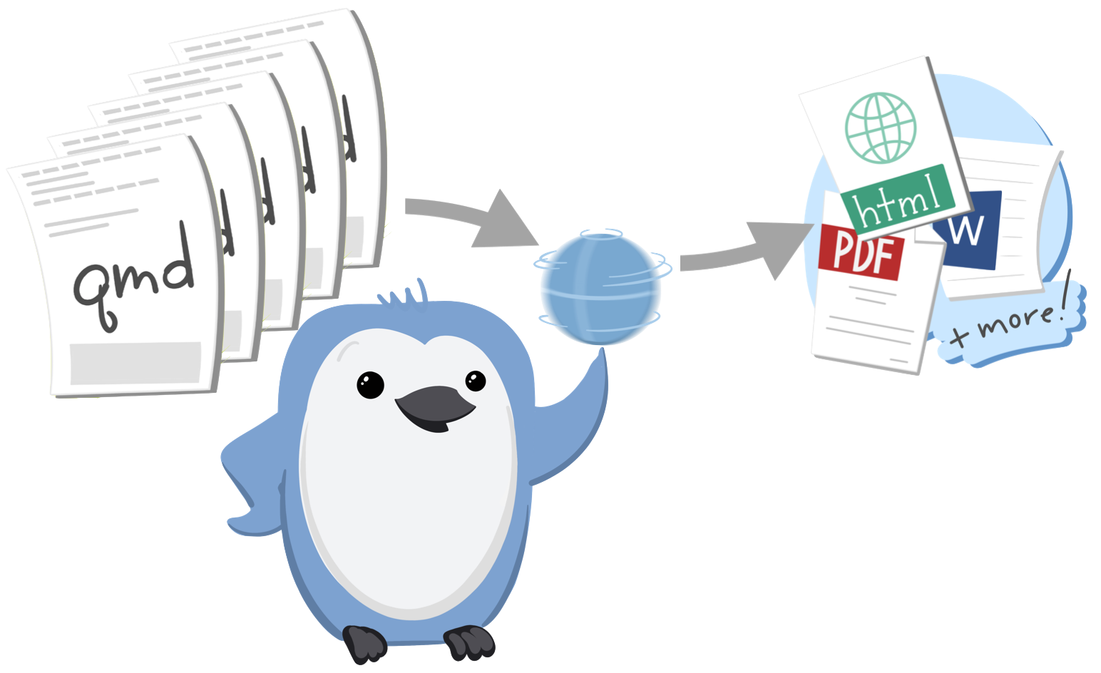
Literate programming can be implemented in different authoring formats. Up until very recently, the most common format for R projects was R Markdown. For Python projects, Jupyter Notebooks remains the standard to date. In this chapter, we will focus on Quarto, a relatively new open-source scientific and technical authoring and publishing system that has the advantage of supporting many different programming languages. This means that code in R, Python, Julia, and other languages can be combined into one document, making project management and collaboration much easier. Quarto also allows us to readily export (or render) our documents to multiple formats such as HTML, PDF, and Word (see Figure 14.1 and Section 14.13).
Literate programming is particularly useful for academic research and data science. Did you know that this entire textbook was written in Quarto? I chose this format because it allows for the seamless combination of explanations with nicely formatted R code and code outputs (i.e. all of the textbook’s tables, data visualisations, quiz questions, etc.). It also automatically generates consistent section and figure numbers, cross-references, bibliographic references, and much more. By the end of this chapter, you’ll be ready to start writing your own term paper, dissertation, thesis, journal article, blog, or presentation slides in Quarto.
Note
Quarto documents are designed to:
Help you collaborate with other researchers (including your future self!) who are interested in both reproducing your results and understanding how you reached them (i.e. the code).
Provide you with a convenient environment in which to do research - a kind of “modern-day lab notebook where you can capture not only what you did, but also what you were thinking” (Wickham, Çetinkaya-Rundel & Grolemund 2023).
Communicate your analyses to others, including those who are not familiar with any programming language.
14.2 Reproducible research
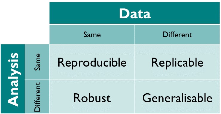
Not only is using Quarto (or any other literate programming format, see Section 14.1) very convenient, it also helps us make our research more reproducible. Unfortunately, the terms reproducible, replicable and repeatable are often confused and, not helping matters, some definitions in the literature contradict each other. In this textbook, we will adopt the terminology of The Turing Way. We thus define reproducibility as the ability of an independent researcher or team to obtain the same results as in a study using the same data and methods as the original study (see Figure 14.2).

This is in contrast to replicability, where the same methods, but different data are used; and robustness, where the same data, but different methods are used. Finally, if a finding can be reliably observed across different datasets with different methods, then we can say that the finding is generalisable.
Given this definition, reproducibility might seem like a low bar to pass. You might be thinking: shouldn’t it be obvious that we’ll get the same results if we repeat a study using exactly the same data and method? Well, yes, it should be. But it very often isn’t! For a start, to be able to even attempt to reproduce the results of a study, the underlying data must be available. Linguists that share their primary data as Ewa Dąbrowska did as part of her 2019 publication (Dąbrowska 2019) remain the exception rather than the norm (see Bochynska et al. 2023)1. Second, the data must be available in an accessible format and must be published together with enough documentation to be understandable to an independent researcher. Third, the author(s) of the original study need to have very diligently documented all their data wrangling and analyses steps. The best way to do this is undoubtedly to use code that does not require closed-source software (e.g. a researcher without a license for SPSS or Stata will not be able to run SPSS or Stata scripts, see Section 1.2). This open code must be shared in an accessible format, too. Fourth, independent researchers need to be able to run these scripts. To this end, it is important that they know exactly which tools were used. Thus, if the analyses were conducted in R, they need to know which R version and which packages and package versions were used (Section 14.10). They also need to know in which order the scripts were run and, finally, the scripts must run on their own computers without any errors. So now, reproducibility doesn’t sound quite so easy, right? Luckily, if we apply the principles of literate programming in Quarto, we can go a long way towards ensuring that our research is reproducible.
NoteGoing further️ 🚀
To find out more about best practices for reproducible research, check out The Turing Way’s excellent Guide for Reproducible Research.
TipYour turn!
Watch this video from 2019, in which Garrett Grolemund (data scientist and instructor at RStudio) explains why literate programming is key to improving medical science, data science, and ultimately all empirical research endeavours. Be aware that everything that Garrett says about R Markdown is also true of Quarto.
Q14.1 What is meant by the replication crisis?2
Q14.2 Which stages of the research process are potential sources of uncertainty?
🐭 Click on the mouse for a hint.
Q14.3 What would it take for a linguist to fully understand the conclusions of another linguist’s quantitative study?
🐭 Click on the mouse for a hint.
14.3 Getting started with Quarto

We will be writing Quarto documents from the RStudio IDE3, which conveniently ships with a version of Quarto, meaning that no additional installation4 is required for you to use Quarto on your computer.
To get started with Quarto:
In RStudio, create a new Project by selecting File > New Project… in the main menu, or by clicking on the “new project” button.
- You can choose the first option to create a new folder for your project if you’ve not yet got one,
- or the second option to select an existing project directory.
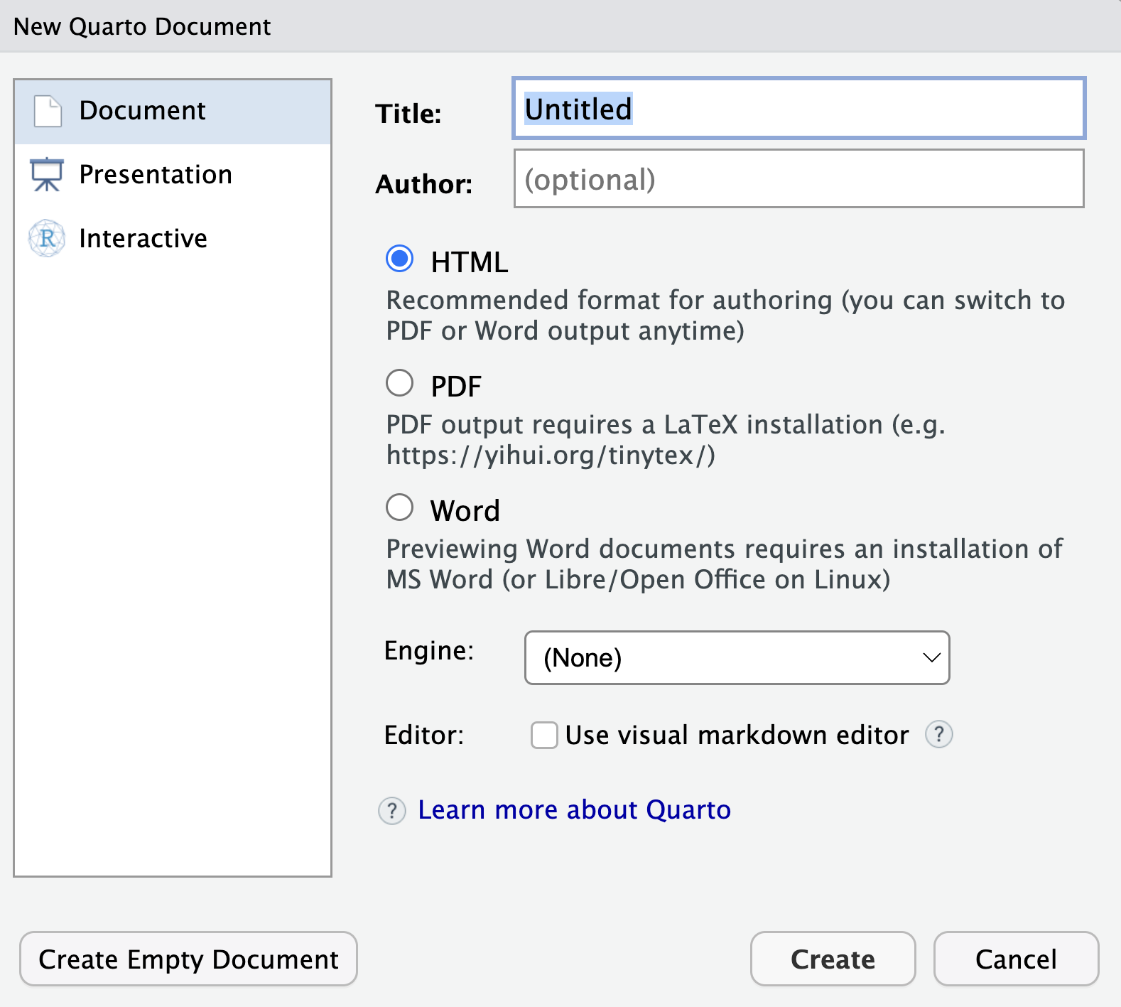
Then, create a new Quarto document by navigating to File > New File > Quarto Document…, or clicking on the “new document” button and selecting “Quarto Document…”. A dialogue menu will appear (Figure 14.3). Leave everything as is and simply click on”Create” at the bottom.
- RStudio has now opened a new, untitled Quarto file (
.qmd). Depending on your settings, this new Quarto document may include some template material, which you can delete. Change the title of your Quarto document (which is not the same as its filename!) and add three further lines to the document header by copying and pasting the following lines at the top of the document, replacing the default header. Quarto document headers5 are written in YAML which, I kid you not, stands for Yet Another Markup Language! 😅
---
title: Learning Quarto
subtitle: "by reproducing the descriptive statistics of Dąbrowska's (2019) study"
author: Write your name here
date: last-modified
---
Click on the “save” button in the menu bar or navigate to File > Save to save your
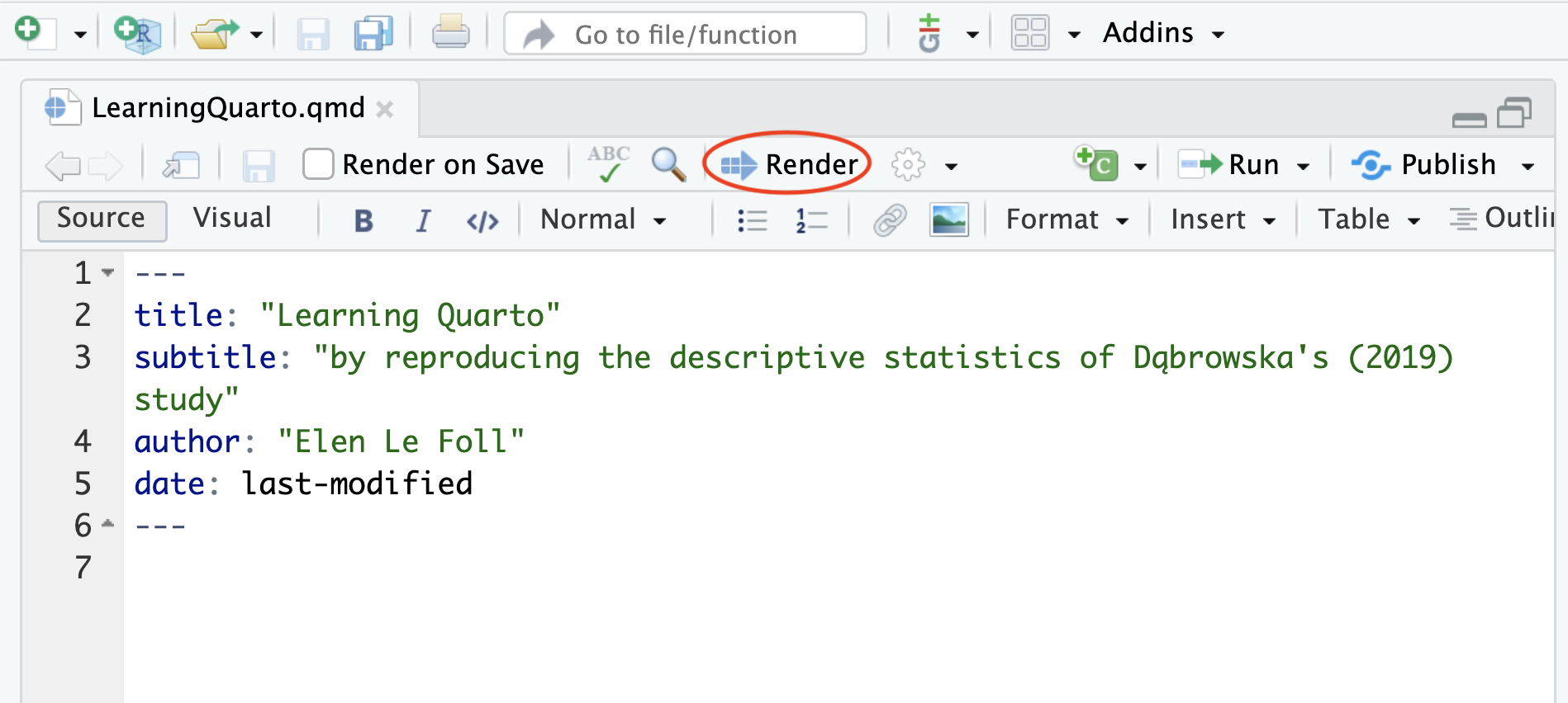
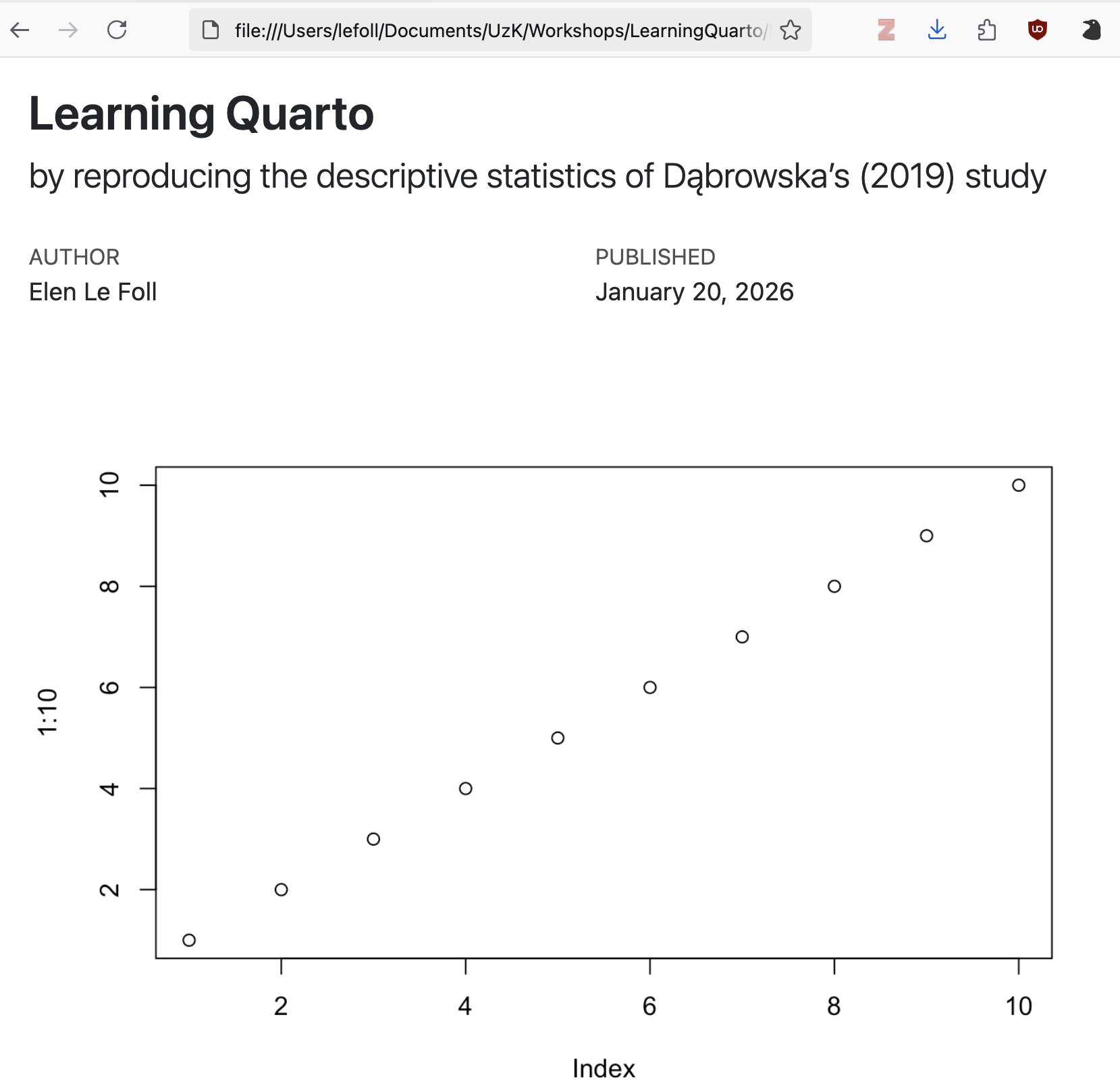
.qmdfile. You will be prompted to give it a name. This could beLearningQuarto.qmd(see Section 3.2 for tips on how to name files).To check your Quarto installation, render your document by either selecting File > Render Document in the main menu, or clicking on “Render” button in the Quarto menu bar (see Figure 14.4). Your
.qmdfile will automatically be rendered to HTML (Quarto’s default rendering format).Navigate to the folder where you saved your
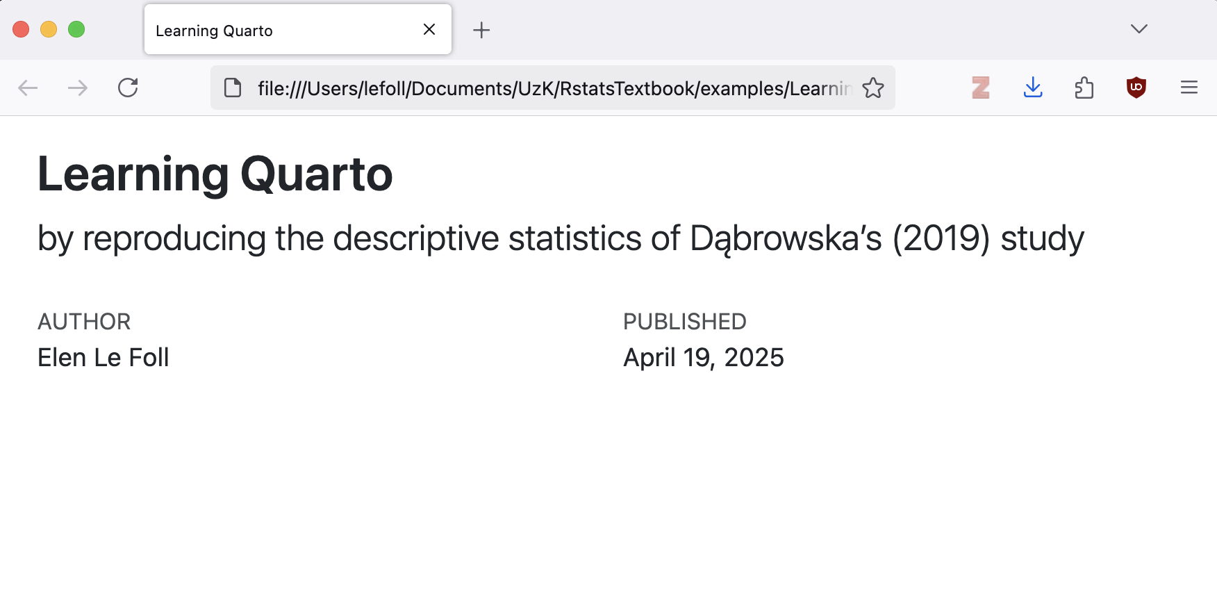
.qmdfile to find the rendered HTML file. You can use a Finder (on macOS) or File Explorer window (on Windows) or go to the “Files” pane in RStudio to do this. The rendered version of your file will have the same filename as your Quarto document, but with the file extension.html(e.g.LearningQuarto.html). If you open on the file, it will appear in your default web browser (e.g. Firefox, Chrome, Safari). You should see that the HTML document features the title of your document, your name as the author, and today’s date (see Figure 14.5).
.qmd file as opened in RStudio
.html file as opened in a web browser
For now, the document is empty. In the next sections, you will learn how to add text, code, and code outputs to your Quarto document.
14.3.1 RStudio’s visual editor
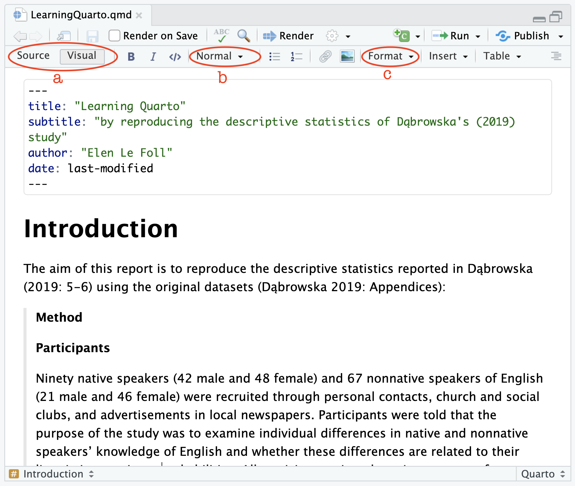
You may have noticed that RStudio proposes two different modes in which Quarto documents can be edited: Source and Visual (see Figure 14.6).

The Visual mode offers a WYSIWYM (What You See Is What You Mean) authoring experience. This means that, in Visual model, you will immediately see the effect of your formatting on screen. For example, to format a word in italics, you can click on the corresponding button in the toolbar (see Figure 14.6) or use the keyboard shortcut — just like you would in text-processing software — and this will immediately display the text in italics.
TipYour turn!
Q14.4 In this task, you will practice using RStudio’s Visual model to format text in a Quarto document.
- In a new line beginning after the final
---of the YAML header, paste the introduction text below. - Using the Quarto editing toolbar, format the text so that, in the Visual mode, it looks like the text displayed in the screenshot below.
- Render the document and compare how it is formatted in the HTML version.
Introduction

The aim of this report is to reproduce the descriptive statistics reported in Dąbrowska (2019: 5-6) using the original datasets (Dąbrowska 2019: Appendix S4):

Method

Participants

Ninety native speakers (42 male and 48 female) and 67 nonnative speakers of English (21 male and 46 female) were recruited through personal contacts, church and social clubs, and advertisements in local newspapers. Participants were told that the purpose of the study was to examine individual differences in native and nonnative speakers’ knowledge of English and whether these differences are related to their linguistic experience and abilities. All participants signed a written consent form before the research commenced.

The L1 participants were all born and raised in the United Kingdom and were selected to ensure a range of ages, occupations, and educational backgrounds. The age range was from 17 to 65 years (M = 38, SD = 16). Twenty-two percent of the participants held manual jobs, 24% held clerical positions, and 28% had professional-level jobs or were studying for a degree; the remaining 26% were occupationally inactive (i.e. unemployed, retired, or homemakers). In terms of education, participants’ backgrounds ranged from no formal qualifications to Ph.D., with corresponding differences in the number of years spent in full-time education (from 10 to 21; M = 14, SD = 2). Six participants reported a working knowledge of another language; the rest described themselves as monolinguals.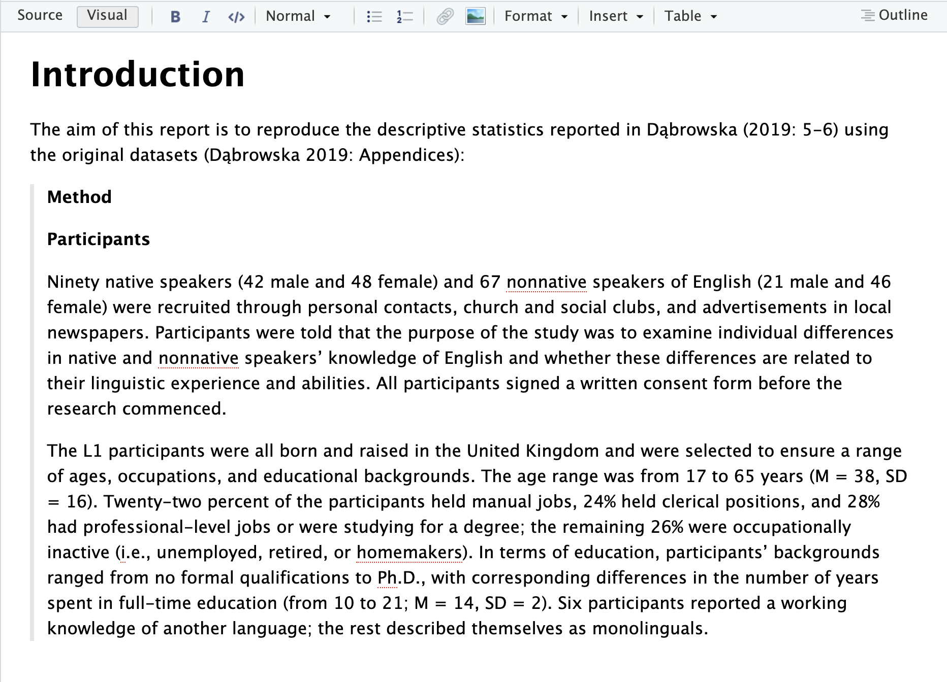
In RStudio’s visual mode, what is the name of the formatting option that indents and adds a grey line to the left of a quoted paragraph as in the screenshot above?
🐭 Click on the mouse for a hint.
NoteClick here for the full solution to Q14.4
In the Visual mode (see Figure 1 (a)), click on the “Normal” drop-down menu (see Figure 1 (b)) to change the formatting of the word Introduction to the “Header 1” style. To format the long citation, choose the “Blockquote” option from the the “Format” drop-down menu (see Figure 1 (c)).
14.4 Markdown text
Writing and formatting text in RStudio’s Visual editor is very similar to writing in a word-processing software such as LibreOffice Writer or Microsoft Word. In the background, however, RStudio automatically converts your formatted text to Markdown in the underlying source code of your .qmd file. Markdown is a plain-text format. For example, in Markdown, words in italics are enclosed in asterisks like this: *italics*. Table 14.1 displays the Markdown syntax for other formatting options commonly used in academic writing.
The best way to get the hang of Markdown is simply to try things out. You will also find a handy cheatsheet under Help > Markdown Quick Reference. Remember that you can always go back to the Visual mode to format your text if that’s easier for you. When it comes to debugging any Quarto syntax errors, however, it’s usually easier to catch these in plain text, so you’ll typically want to switch to the Source mode for that.
TipYour turn!
Switch to the Source mode to view the text that you formatted in the Visual editor for Q14.4 in Markdown format.
Q14.5 How is text highlighted in bold displayed in Markdown?
Q14.6 How is a first-level heading displayed in Markdown?
Q14.7 How are block quotes formatted in Markdown?
Q14.8 How will the word ~~mystery~~ be formatted in Markdown?
Note
Markdown is gaining in popularity and is now widely supported across many platforms, from text editors to content management systems, ensuring that your formatting remains consistent and portable. Whether you’re writing documentation, creating blog posts, or taking notes, Markdown’s simplicity and versatility make it a valuable skill to have beyond academic writing and Quarto.
You can learn more about Markdown here: https://www.markdownguide.org/basic-syntax/.
Markdown is gaining in popularity and is now widely supported across many platforms, from text editors to content management systems, ensuring that your formatting remains consistent and portable. It’s increasingly used to write documentation, blog posts, or simply to take notes. Check out the Markdown Guide to learn more.
| Markdown syntax | Rendered output |
|---|---|
*italics* |
italics |
**bold** |
bold |
***bold italics*** |
bold italics |
superscript^2^ / subscript~2~ |
superscript2 / subscript2 |
~~strikethrough~~ |
|
`verbatim code` |
verbatim code |
# Heading 1 |
Heading 1 |
## Heading 2 |
Heading 2 |
### Heading 3 |
Heading 3 |
<https://quarto.org> |
https://quarto.org |
[Quarto guide](https://quarto.org) |
Quarto guide |
|
|
|
|
Note
To make writing in Quarto more convenient and less error-prone, you can switch on a spell-checker within RStudio. To do so, go to Tools > Global Options… > Spelling. You may need to restart RStudio for the change to take effect.
14.5 Code chunks
To run code inside a Quarto document, we need to insert a code chunk. There are three ways to do so:
- Using the keyboard shortcut
- Clicking on the green “Insert chunk” button icon in the editor toolbar
- Manually typing the chunk delimiters
```{r}and```
It is definitely worth learning the keyboard shortcut as it will save you a lot of time in the long run!
In the code chunk below, {r} tells Quarto that this chunk is written in the programming language R. If we wanted to embed a chunk of Python code, we must begin it with ```{python} instead.
Using one of the three aforementioned options, insert the following R code chunk in your document.
```{r}
library(here)
library(tidyverse)
```
To run code within a Quarto document, we can either run:
- each individual line of code using the keyboard shortcut or
- the entire code chunk either by clicking the “Run”
 icon or with shortcut .
RStudio will execute the code and display the results either within your document (below each chunk) or in the Console, depending on your RStudio settings.6
Chunk output can be customised with chunk options. There are many options to choose from, but the most important options control whether a code block should be executed when the Quarto document is rendered and what results are inserted in the rendered version:
eval: falseprevents code from being evaluated. Given that the code is not run, no code outputs are generated either.include: falseruns the code, but does not show the code or its outputs in the rendered document. This option is useful for code chunks that are not informative to the readers of your document.echo: falseprevents the code from appearing in the rendered document, but displays the code outputs. This option is useful when you want to present the results of your analyses to people who are not interested in the underlying code.message: falseorwarning: falseprevents messages or warnings from appearing in the rendered document.
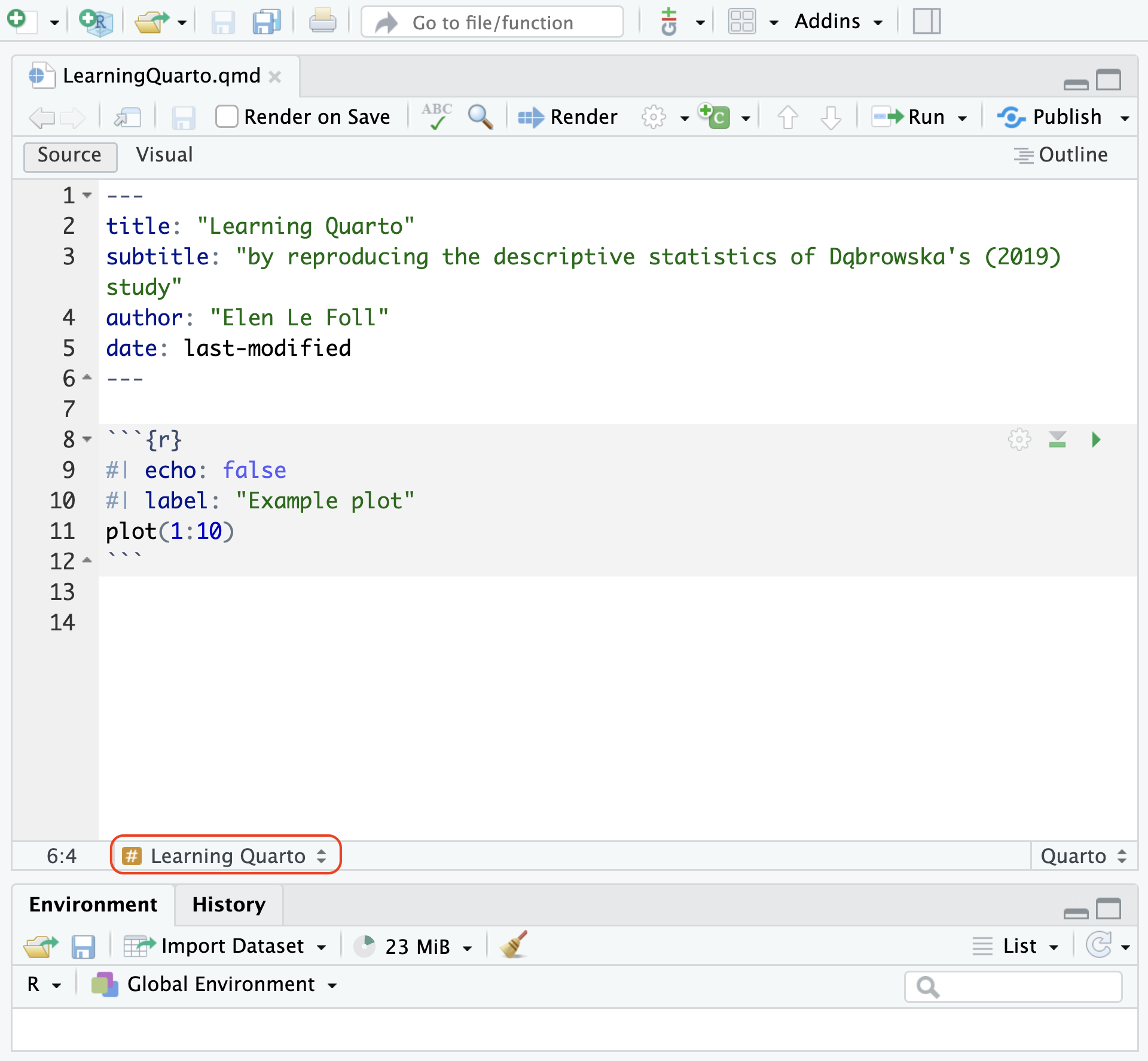
It is also possible to label code chunks using the label option (see code chunk below). This can help to navigate long Quarto documents using the drop-down menu available in the bottom-left corner of the Source pane (see Figure 14.8). It also helps to quickly identify which code chunk is causing errors during rendering. Chunk labels should be short but meaningful.
```{r}
#| echo: false
#| label: "Example plot"
plot(1:10)
```
In RStudio the easiest way to set a chunk option is by clicking the gear icon in the top right corner of the chunk that you want to modify. This way, you can both choose a label and set chunk options. If you prefer to write code chunk options manually, these are placed at the top of the corresponding chunk following #|, as in the chunk above and Figure 14.8. As you can see in Figure 14.9, the echo: false chunk option means that the rendered document includes the chunk output, but not the code itself.
TipYour turn!
In your Quarto document, add a label to your first R chunk and render your document to HTML.
```{r}
#| label: setup

library(here)
library(tidyverse)
```
Q14.9 What is the output of the setup chunk in your rendered .html document?
🐭 Click on the mouse for a hint.
Q14.10 Which code chunk option can you use to remove the two messages from the rendered version of your Quarto document, whilst still ensuring that the setup chunk is displayed and executed so that the libraries can be used in future code chunks?
🐭 Click on the mouse for a hint.
Q14.11 Which code chunk option can you use to remove both the setup chunk and its outputs from the rendered version of your Quarto document, whilst still ensuring that the libraries are loaded so that their functions can be used further down in the document?
🐭 Click on the mouse for a hint.
14.6 Inline code
So far, we have seen how we can insert and format text in Quarto and how we can add code chunks with various options. But, to make the most of literate programming, we want to combine the two.
WarningPrerequisites
This chapter assumes that you are familiar with the following research article (which was first introduced in Section 6.1):
Dąbrowska, Ewa. 2019. Experience, Aptitude, and Individual Differences in Linguistic Attainment: A Comparison of Native and Nonnative Speakers. Language Learning 69(S1). 72-100. https://doi.org/10.1111/lang.12323.
Our starting point for this chapter are the author’s original datasets, which are linked in the article’s Appendix S4.
Appendix S4: Datasets
Dąbrowska, E. (2018). L1 data [Data set]. Retrieved from https://www.iris-database.org/iris/app/home/detail?id=york:935513
Dąbrowska, E. (2018). L2 data [Data set]. Retrieved from https://www.iris-database.org/iris/app/home/detail?id=york:935514
You will only be able to reproduce the analyses and answer the quiz questions from this chapter if you have successfully imported these two two datasets. To do so, follow the instructions from Section 6.3 to Section 6.5 and complete Q6.8—Q6.12.
Alternatively, you can download Dabrowska2019.zip from the textbook’s GitHub repository, which contains both datasets. To launch the project correctly, first unzip the file and then double-click on the Dabrowska2019.Rproj file.
Insert the following R chunk to load the Dąbrowska (2019) data so that they may be used in your Quarto document. As this import-data chunk requires the here() function, it must come after the setup chunk because, when the document is rendered, code chunks will be executed in the order that they appear. If the {here} library is not loaded before the data are imported, the rendering process will be aborted and an error message will be displayed in the Console.
```{r}
#| label: import-data
#| include: false

L1.data <- read.csv(file = here("data", "L1_data.csv"))
L2.data <- read.csv(file = here("data", "L2_data.csv"))
```
To begin, we will reproduce the following basic descriptive statistics about the two datasets:
“Ninety native speakers (42 male and 48 female) and 67 nonnative speakers of English (21 male and 46 female) were recruited through personal contacts, church and social clubs, and advertisements in local newspapers” (Dąbrowska 2019: 5).
As you may recall from Chapter 7, the number of native and non-native participants corresponds to the number of rows in the corresponding dataset:
nrow(L1.data)[1] 90nrow(L2.data)[1] 67In Quarto, we can use inline code to dynamically insert these numbers into our paragraph. Inline code in R begins with `{r} and ends with a single backtick `. It is best to use the Source mode to insert inline code. Using the Source mode, add the following section to your Quarto document and render it to HTML.
## Descriptive statistics about the participants

 `{r} nrow(L1.data)` native speakers and `{r} nrow(L2.data)` nonnative speakers of English were recruited through personal contacts, church and social clubs, and advertisements in local newspapers.
The rendered version should read like this (if you are obtaining different numbers, this either means that you have tempered with the original data files or that they have been corrupted)7:
Descriptive statistics about the participants
90 native speakers and 67 nonnative speakers of English were recruited through personal contacts, church and social clubs, and advertisements in local newspapers.
Inline code should only be used for very simple code, ideally with no more than one function, as in `{r} nrow(L1.data)`. To insert the output of more complex operations, it is best to write the code and save its output(s) to the local environment in a hidden code chunk (using the option #| include: false, see Section 14.5).
```{r}
#| label: L1-gender
#| include: false

L1.males <- L1.data |>
  filter(Gender == "M") |>
  count()

L1.females <- L1.data |>
  filter(Gender == "F") |>
  count()
```
The saved objects (L1.males and L1.females) each contain one number. They can therefore be directly called within the text as inline code:
`{r} nrow(L1.data)` native speakers (`{r} L1.males` male and `{r} L1.females` female) and `{r} nrow(L2.data)` nonnative speakers of English were recruited through personal contacts, church and social clubs, and advertisements in local newspapers.When rendered, the paragraph will read:
90 native speakers (42 male and 48 female) and 67 nonnative speakers of English were recruited through personal contacts, church and social clubs, and advertisements in local newspapers.
TipYour turn!
Q14.12 In your Quarto document, add a code chunk called L2-gender in which you compute the values necessary to complete the missing descriptive statistics in the sentence above. When rendered, your sentence should read:
90 native speakers (42 male and 48 female) and 67 nonnative speakers of English (21 male and 46 female) were recruited through personal contacts, church and social clubs, and advertisements in local newspapers.
Which value requires more than just one line of code?
🐭 Click on the mouse for a hint.
NoteClick here for the solution to Q14.12
To save the number of male L2 participants as an R object, we can follow the same procedure as above.
L2.males <- L2.data |>
  filter(Gender == "M") |>
  count()
For the number of female L2 participants, however, it’s not so simple because some are labelled f, while others are labelled F (see Section 9.4.2).
table(L2.data$Gender)
 f  F  M
 6 40 21
Below are four possible methods to solve this issue (and there are many more still!):
# Method 1:
L2.Females <- L2.data |>
  filter(Gender == "F") |>
  count()

L2.females <- L2.data |>
  filter(Gender == "f") |>
  count()

L2.allfemales <- L2.Females + L2.females

# Method 2:
L2.allfemales <- L2.data |>
  filter(Gender == "F" | Gender == "f") |>
  count()

# Method 3:
L2.allfemales <- L2.data |>
  filter(Gender %in% c("F", "f")) |>
  count()

# Method 4:
L2.allfemales <- L2.data |>
  mutate(Gender = toupper(Gender)) |>
  filter(Gender == "F") |>
  count()
Some of these methods are perhaps more elegant than others, but they are all acceptable. After all, they all work! 🙃
Once they are saved to the local environment, the values can be inserted inline in the usual way:
`{r} nrow(L1.data)` native speakers (`{r} L1.males` male and `{r} L1.females` female) and `{r} nrow(L2.data)` nonnative speakers of English (`{r} L2.males` male and `{r} L2.allfemales` female) were recruited through personal contacts, church and social clubs, and advertisements in local newspapers. If we want to start our paragraph with 90 written in as a word rather than in digits, we can use the numbers_to_words function() function from the {xfun} package. First, you’ll need to install the {xfun} package and then add a line to your setup chunk to load it.8
```{r}
#install.packages("xfun")
library(xfun)
```
First, let’s test that the package works by running the following line of code from the Console:
numbers_to_words(nrow(L1.data))[1] "ninety"To start our paragraph with a capital letter, we’ll need to set the function’s cap argument to TRUE.
`{r} numbers_to_words(nrow(L1.data), cap = TRUE)` native speakers (`{r} L1.males` male and `{r} L1.females` female) and `{r} nrow(L2.data)` nonnative speakers of English...Next, we want to reproduce the following descriptive statistics about the L1 participants:
“The L1 participants were all born and raised in the United Kingdom and were selected to ensure a range of ages, occupations, and educational backgrounds. The age range was from 17 to 65 years (M = 38, SD = 16)” (Dąbrowska 2019: 5).
We can use the base R functions min(), max(), mean(), and sd() to compute these values.
The L1 participants were all born and raised in the United Kingdom and were selected to ensure a range of ages, occupations, and educational backgrounds. The age range was from `{r} min(L1.data$Age)` to `{r} max(L1.data$Age)` years (*M* = `{r} mean(L1.data$Age)`, *SD* = `{r} sd(L1.data$Age)`).The rendered document will read:
The L1 participants were all born and raised in the United Kingdom and were selected to ensure a range of ages, occupations, and educational backgrounds. The age range was from 17 to 65 years (M = 37.5444444, SD = 16.148998).
Whilst these values are correct, in practice, we want to round them off to the nearest integer. To this end, we can wrap the round() function around the mean() and sd() function (see Section 7.5.1).
The L1 participants were all born and raised in the United Kingdom and were selected to ensure a range of ages, occupations, and educational backgrounds. The age range was from `{r} min(L1.data$Age)` to `{r} max(L1.data$Age)` years (*M* = `{r} round(mean(L1.data$Age))`, *SD* = `{r} round(sd(L1.data$Age))`).The rendered document will read:
The L1 participants were all born and raised in the United Kingdom and were selected to ensure a range of ages, occupations, and educational backgrounds. The age range was from 17 to 65 years (M = 38, SD = 16).
TipYour turn!
👩🏾💻 Copy the code and text sections corresponding to the description of participants’ professional occupations and education displayed Section 14.6 (in the textbox “More complex inline computations”) into your Quarto document and render it to HTML. Compare the values in your rendered document with the original ones from the published study (see below).
“Twenty-two percent of the participants held manual jobs, 24% held clerical positions, and 28% had professional-level jobs or were studying for a degree; the remaining 26% were occupationally inactive (i.e. unemployed, retired, or homemakers). In terms of education, participants’ backgrounds ranged from no formal qualifications to Ph.D., with corresponding differences in the number of years spent in full-time education (from 10 to 21; M = 14, SD = 2). Six participants reported a working knowledge of another language; the rest described themselves as monolinguals” (Dąbrowska 2019: 6).
Q14.13 Compare the rendered version of your document with the original descriptive statistics reported in Dąbrowska (2019: 6). Could you successfully reproduce these descriptive statistics? Which values are different?
NoteCounting words
If you need to adhere to a specific word count, RStudio has a useful function to count the number of words you have written, excluding the YAML header and all code chunks. In RStudio’s top menu, click on “Edit” and select “Word Count” to find out how many words you’ve written so far.
You may also want to check out Andrew Heiss’ Quarto extension that computes different types of word counts (e.g. including or excluding references) and optionally prints them in the rendered versions of your Quarto documents.
14.7 Tables
The easiest way to manually construct a table in a Quarto document in RStudio is to switch to Visual mode and click on Insert > Table. You can choose how many rows and columns you need and then fill in your table in the Visual editor.
| Same data | Different data | |
|---|---|---|
| Same analysis method | Reproducible | Replicable |
| Different analysis method | Robust | Generalisable |
When you switch to the Source mode, you will see that, in Markdown (see Section 14.4), your table has been converted to a pipe table. Pipe tables allow for column alignment and captions.
|                               | Same data    | Different data |
|-------------------------------|--------------|----------------|
| **Same analysis method**      | Reproducible | Replicable     |
| **Different analysis method** | Robust       | Generalisable  |

: Terminology used in this chapter
Most of the time, however, you will want to display tabular results based on data that you have imported, wrangled, and/or analysed in R. If the output of a code chunk within your Quarto document is a table, it will be displayed in your rendered document by default (unless you specify a chunk option to hide its output, see Section 14.5).
L1.data |>
  count(OtherLgs,
        sort = TRUE)
OtherLgs n
1 None 84
2 German 3
3 French 2
4 Spanish 1However, this output is not particularly nicely formatted. There are several R packages designed to create tables that are “presentation-ready”. One of these is the {gt} package. Beyond its main function gt(), it offers many more functions to further style tables such as cols_label() to change the column headers. You will need to install this package before you can use it (see Section 14.10).
```{r}
#| label: tbl-L1-languages
#| tbl-cap: "Example of a {gt} table"
#| tbl-cap-location: top
#| tbl-colwidths: [80,20]

#install.packages("gt")
library(gt)

L1.data |>
  count(OtherLgs,
        sort = TRUE) |>
  gt() |>
  cols_label(
    OtherLgs = "Additional language",
    n = "N")
```| Additional language | N |
|---|---|
| None | 84 |
| German | 3 |
| French | 2 |
| Spanish | 1 |
In addition, Quarto also has a range of chunk options to customise the display of tables, including tbl-cap for the addition of a table caption and tbl-cap-location to determine where the caption is placed. Note that, in the above chunk, the table’s label chunk option begins with tbl-. This allows for in-text cross-referencing to the table with the insertion of @tbl-L1-languages within the text of the Quarto document, which will automatically be rendered as the following linked and numbered cross-reference: Table 14.2.
NoteGoing further 🚀
The Quarto guide provides further information about formatting tables: https://quarto.org/docs/authoring/tables.html.
14.8 Figures
In Quarto documents, figures can either be inserted from image files (e.g. .png or .jpeg files, see Section 2.3) or from the output of a code chunk (e.g. a plot, see Chapter 10).
14.8.1 Images
To embed an image from an external file, you can use the “Insert” menu in RStudio’s Visual editor and select “Figure / Image” (see Figure 14.10). This will open up a menu where you can select the image that you want to insert, as well as add alt-text (see Section 10.1.3) and a caption. The easiest way to adjust the size of an embedded image is to click on the image and then adjust the size of the image with the blue circle in the bottom-right corner of the image (see Figure 14.10).
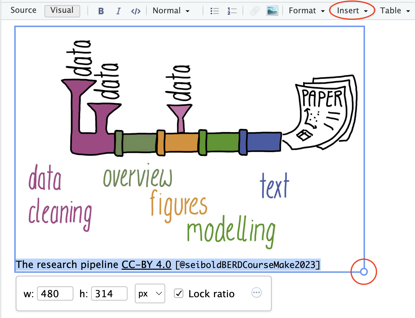
Below is the source code for Figure 14.11 in Markdown. The code includes the relative path to the image file (see Section 3.3) relative to the project directory (see Section 6.3). In the example below, the image file BERD_pipeline-real.jpg is located in a subfolder called images. If you want to try this out yourself, you will need to create this subfolder within your own project directory and save Figure 14.11 to this subfolder.
 @seiboldBERDCourseMake2023]](images/BERD_pipeline-real.jpg){#fig-RealisticPipeline fig-alt="Cartoon drawing of a complex set of pipes with various entry points for \"data\" and a single output: a research paper with text, a table, and a plot. Sections of the pipe are coloured according to the processes that they correspond to. These include data cleaning, overview, figures, modelling, and text." width="480"}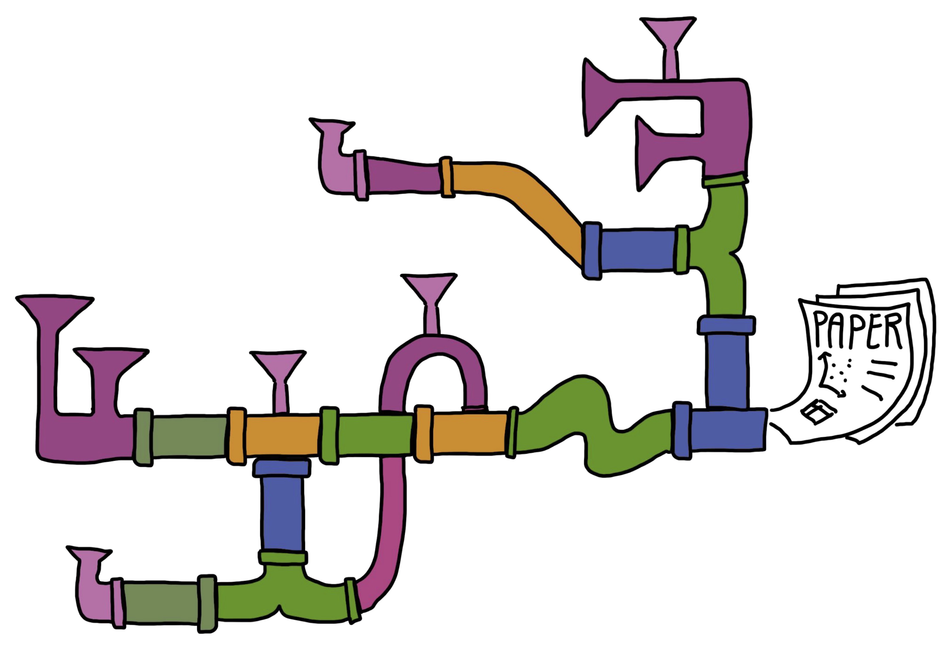
This example embedded image includes a caption (that, itself, includes a link), an alt-text (see Section 10.1.3), and a custom width in pixel. Note that, in the source code, special characters such as quotation marks need to be escaped using a backslash \. Tags beginning with #fig- can be used to cross-reference images by replacing the # with @. Hence, in this chapter, @fig-RealisticPipeline in the Quarto source code is rendered as Figure 14.11.
Figures can be arranged in many ways. The example below uses the ::: div syntax to display two images side-by-side. This syntax also allows for subcaptions as shown in Figure 14.12.
::: {#fig-Pipelines layout-ncol="2"}
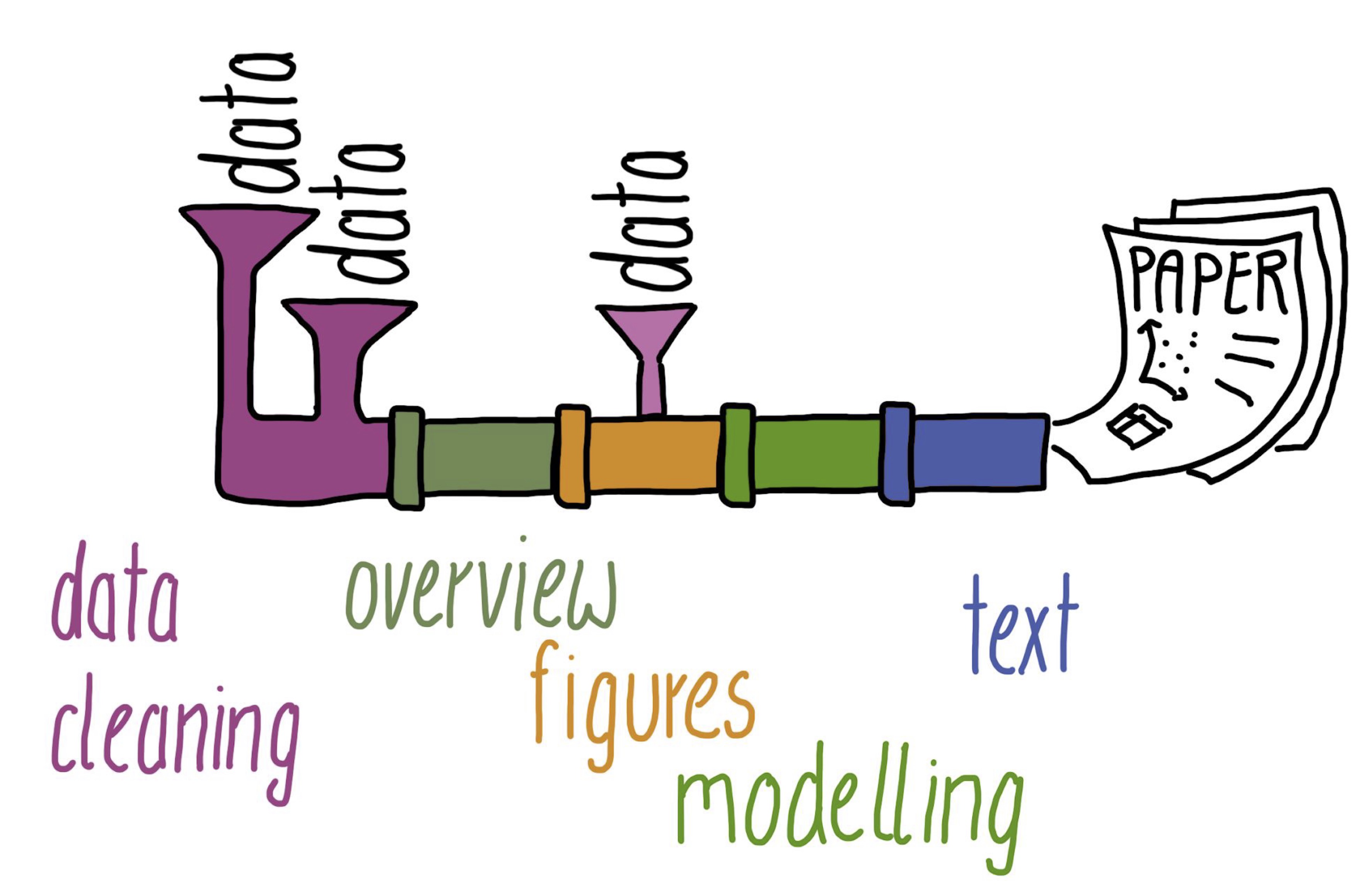{#fig-IdealisedPipeline}
{#fig-RealisticPipeline2}
Research workflows as pipelines [[CC BY 4.0](https://creativecommons.org/licenses/by/4.0/) @seiboldBERDCourseMake2023]
:::
NoteGoing further 🚀
To find out more about inserting and arranging figures, check out the detailed Quarto guide: https://quarto.org/docs/authoring/figures.html.
14.8.2 Plots
If your Quarto document includes code chunks that generate plots, they will automatically be integrated in your rendered document. Plots will either appear immediately after the corresponding code chunk or where the code chunk would be, if you chose to hide the code chunk that generated the plot with the echo: false option.
As with computed tables (see Section 14.7), various code chunk options can be added to customise the look of computed figures in rendered documents. Compare the code chunk options below and the generated output in Figure 14.13.
```{r}
#| label: fig-scatterplot
#| fig-cap: "L2 participants' lexical proficiency in English and their professional occupational group"
#| fig-height: 5
#| fig-asp: 0.618
#| message: false

L2.data |>
  ggplot(mapping = aes(x = VocabR,
                       y = CollocR)) +
  geom_point(aes(colour = OccupGroup),
             size = 2) +
  geom_smooth(method = "lm") +
  scale_colour_viridis_d() +
  labs(x = "Vocabulary test scores",
       y = "Collocation test scores",
       colour = "Occupational\ngroups") +
  theme_bw()
```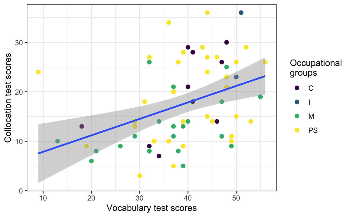
According to the authors of “R for Data Science”, figure sizing and scaling in R is “an art and science and getting things right can require an iterative trial-and-error approach” (Wickham, Çetinkaya-Rundel & Grolemund 2023). This is because there are five main options that control figure sizing: fig-width, fig-height, fig-asp, out-width and out-height. The first three control the size of the figure created by R, whereas the latter two control the size at which it is inserted in the rendered document.
If you are sharing your research analyses and results in HTML format, you can also embed interactive plots (see Section 10.2.8) in your Quarto documents. In HTML format, it is therefore possible to hover over Figure 14.14 to explore the data interactively.
Show R code to generate the interactive plot below.
#install.packages("plotly")
library(plotly)

L2.scatter2 <- L2.data |>
  ggplot(mapping = aes(x = VocabR,
                       y = CollocR,
                       text = paste("L1:", NativeLg, "</br>Age:", Age, "</br>Years in formal education:", EduTotal, "</br>Job:", Occupation))) +
  geom_point(aes(colour = OccupGroup),
             size = 2) +
  scale_colour_viridis_d() +
  labs(x = "Vocabulary test scores",
       y = "Grammar test scores",
       colour = "Occupational\ngroups") +
  theme_bw()

ggplotly(L2.scatter2)14.9 References
An important aspect of academic writing is the inclusion of in-text bibliographic references (citations) and a well-formatted list of references (also referred to as a bibliography). RStudio’s Visual editor makes inserting bibliographic references very convenient. To insert a reference, click on “Insert” and then select “Citation” or use the keyboard shortcut .This opens up a menu (see Figure 14.15) giving you the option to search for the source that you’d like to cite on your own computer (e.g. in your own Zotero database, if you use Zotero), via the Crossref database, or directly using a DOI.
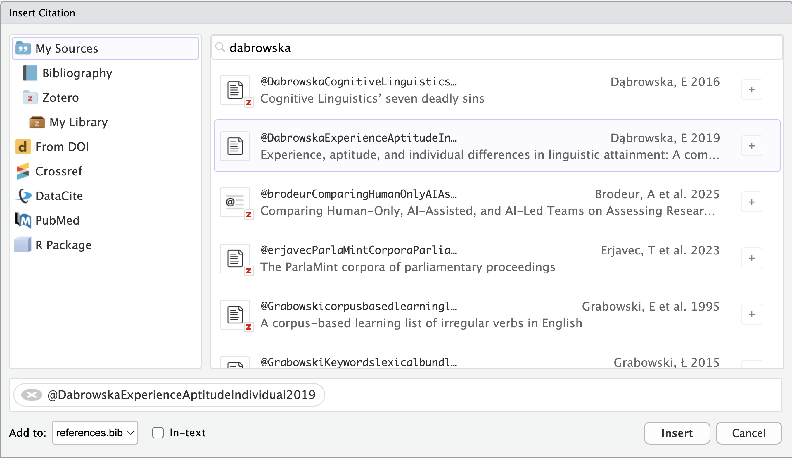
Alternatively, if you start typing @ in the Visual editor, a quick reference menu will appear. Either way, any references that you add will be displayed as @ followed by a reference identifier. For example, in the source code of this Quarto document, every reference to Dąbrowska (2019) is indicated as @DabrowskaExperienceAptitudeIndividual2019.
Note
For more information on how to format your in-text citations, see the Quarto guide.
When you insert your first reference in a Quarto document, RStudio will automatically create a references.bib file in your project folder. All references are automatically added to this new BibLaTeX file. As shown below, .bib files contain entries that begin with @ followed by the type of reference (article, book, manual, url, etc.) and the reference identifier (e.g. DabrowskaExperienceAptitudeIndividual2019, wickhamDataScienceImport2023). The rest of the entries contains structured information about each reference including its title, date of publication, and DOI or ISBN.
references.bib
@article{
  DabrowskaExperienceAptitudeIndividual2019,
  title={Experience, Aptitude, and Individual Differences in Linguistic Attainment: A Comparison of Native and Nonnative Speakers},
  volume={69},
  ISSN={1467-9922},
  url={https://onlinelibrary.wiley.com/doi/abs/10.1111/lang.12323},
  DOI={10.1111/lang.12323},
  number={S1},
  journal={Language Learning},
  author={Dąbrowska, Ewa},
  year={2019},
  pages={72–100}
}

@book{
  wickhamDataScienceImport2023,
  place={Beijing, Boston, Farnham, Sebastopol, Tokyo},
  edition={2},
  title={R for Data Science: Import, tidy, transform, visualize, and model data},
  ISBN={978-1-4920-9740-2},
  url={https://r4ds.hadley.nz/},
  publisher={O’Reilly},
  author={Wickham, Hadley and Çetinkaya-Rundel, Mine and Grolemund, Garrett},
  year={2023}
}
In order to connect this bibliography.bib file with our Quarto document, we need to add a bibliography key to our YAML header (see Section 14.3). Provided that our references.bib file is located in the same folder as our Quarto document (which is what RStudio does by default), we can simply add the following line to our document header:
---
title: Learning Quarto
subtitle: "by reproducing the descriptive statistics of Dąbrowska's (2019) study"
author: Elen Le Foll
date: last-modified
bibliography: references.bib
---
With this modified YAML header, when the document is rendered, a bibliography will automatically be added to the end of the document. This means that, if you have citations in your document, it is a good idea to include a header section # References at the end of the document.
References
Dąbrowska, Ewa. 2019. “Experience, Aptitude, and Individual Differences in Linguistic Attainment: A Comparison of Native and Nonnative Speakers.” Language Learning 69 (S1): 72-100. https://doi.org/10.1111/lang.12323.
Wickham, Hadley, Mine Çetinkaya-Rundel, and Garrett Grolemund. 2023. R for Data Science: Import, Tidy, Transform, Visualize, and Model Data. 2nd ed. O’Reilly. https://r4ds.hadley.nz/.
By default, Quarto will use the Chicago Manual of Style author-date citation format (as above). However, we can point to a different citation stylesheet in the form of a .csl (Citation Style Language) file in the YAML header. This allows us to determine exactly how our bibliography and in-text citations should be formatted. Many institutions, publishers, and journals have their own (sometimes annoyingly specific!) requirements. Luckily, the open-source research community has put together a large repository of citation stylesheets for you to choose from: https://www.zotero.org/styles. You can download any of these stylesheets (as a .csl file), place the file in your project folder, and then link it to your Quarto document by adding a cls key to your header.
---
title: Learning Quarto
subtitle: "by reproducing the descriptive statistics of Dąbrowska's (2019) study"
author: Elen Le Foll
date: last-modified
bibliography: references.bib
csl: international-journal-of-learner-corpus-research.csl
---
For example, if you wanted to submit your paper to the International Journal of Learner Corpus Research, you can download the corresponding CLS stylesheet from the Zotero styles database, save it in your project folder, and link to it in your YAML header as above. When rendered, your document’s bibliography will then read:
References
Dąbrowska, E. (2019). Experience, Aptitude, and Individual Differences in Linguistic Attainment: A Comparison of Native and Nonnative Speakers. Language Learning, 69(S1), 72-100. https://doi.org/10.1111/lang.12323.
Wickham, H., Çetinkaya-Rundel, M., & Grolemund, G. (2023). R for data science: Import, tidy, transform, visualize, and model data (2nd ed.). O’Reilly. Retrieved from https://r4ds.hadley.nz/.
TipYour turn!
Using any of the methods described above, add an in-text bibliographic reference to the following article in your Quarto document:
In’nami, Yo, Atsushi Mizumoto, Luke Plonsky & Rie Koizumi. 2022. Promoting computationally reproducible research in applied linguistics: Recommended practices and considerations. Research Methods in Applied Linguistics 1(3). 100030. https://doi.org/10.1016/j.rmal.2022.100030.
Specifically, we want to cite this passage from page 8:
As implementing these steps may seem daunting, we recommend that researchers engage in reproducible research incrementally. That may be one small step for a researcher, but it will represent a giant leap for the field of applied linguistics when consolidated and accumulated in the long run.
Q14.14 If the key to this article in the .bib file is innami2022, which in-text citation can be used to cite this specific page within a Quarto document?
🐭 Click on the mouse for a hint.
Go to the Zotero style repository and download the .csl citation stylesheet to format references according to the American Psychological Association (APA) 7th edition. Link this stylesheet to your Quarto document and render to HTML.
Q14.15 Now that your document includes references formatted in APA7, how are the authors’ names listed in your bibliography?
NoteLiterature management 📚
Managing the large number of references that we need to consult, read, and cite when doing research can be a real challenge. The good news is that reference management software are there to help you overcome this challenge! Whether you are working on a term paper, a Master’s dissertation, PhD thesis, or post-doctoral project, it is always worth investing the time to learn to use a reference manager!
Zotero is a free and open-source bibliographic reference manager that will help you organise all your sources and generate beautifully formatted bibliographies for all your projects. It offers various browser extensions that enable you to quickly add references to your library directly from your web browser.
What’s more, Zotero can be integrated in RStudio, making it very easy to include BibTeX-formatted references in your Quarto documents. Find out more in the RStudio documentation.
Combining Zotero and Quarto also allows you to generate annotated bibliographies. Benjamin Tjepkes explains how to do this in a detailed blog post.
![]()
14.10 Computing environment
In addition to referencing academic papers, it is also very important that we reference which R version we used for our analyses and which packages and package versions. This serves two purposes:
- Independent researchers (and our future selves!) know exactly what they need to be able to reproduce our analyses (see Section 14.2).
- We give credit to the kind people who spent time and effort developing and sharing the
Rpackages that we used for our analyses (see Section 1.2).
The easiest way to “give credit where credit is due” to R package developers is to use the {grateful} package. Its cite_packages() function will scan your project for all the R packages that are used and generate a BibTeX file called grateful-refs.bib that contains the package references. Having first installed the package, load the {grateful} library:
#install.packages("grateful")
library(grateful)
Make sure that all the packages that your script relies on are loaded and then run the following command once to generate a bibliography of all loaded packages:
cite_packages(out.dir = getwd(),
              omit = NULL)
The .bib text generated by the {grateful} library should now be in your Quarto project directory. Next, add a reference to this BibTeX file in your YAML header. This means that your Quarto document will now have be linked to two bibliography files, which is fine as long as you use the following YAML syntax to reference them both (watch the indentation!):
---
bibliography:
  - references.bib
  - grateful-refs.bib
---
We can now call the cite_packages(output = "paragraph") function to generate a paragraph that mentions all the packages used in the document and add their references to the bibliography (either at the bottom of your rendered Quarto document or in a specific References section as in this textbook).
cite_packages(output = "paragraph",
              out.dir = getwd(),
              pkgs = "Session",
              omit = NULL)
We used R v. 4.5.2 (R Core Team 2025) and the following R packages: checkdown v. 0.0.13 (Moroz 2020), grateful v. 0.3.0 (Rodriguez-Sanchez & Jackson 2025), gt v. 1.2.0 (Iannone et al. 2025), here v. 1.0.2 (Müller 2025), plotly v. 4.11.0 (Sievert 2020), tidyverse v. 2.0.0 (Wickham et al. 2019), webexercises v. 1.1.0 (Barr & DeBruine 2023), xfun v. 0.55 (Xie 2025).
Alternatively, cite_packages() can generate a table with all the package names, versions, and references. Table 14.3 lists the packages used in this chapter. To display functioning links and references, the table is rendered using the kable() function from the {knitr} package.
#install.packages("knitr")
pkgs <- cite_packages(output = "table",
                      out.dir = getwd(),
                      omit = NULL)
knitr::kable(pkgs)| Package | Version | Citation |
|---|---|---|
| base | 4.5.2 | R Core Team (2025) |
| checkdown | 0.0.13 | Moroz (2020) |
| grateful | 0.3.0 | Rodriguez-Sanchez & Jackson (2025) |
| gt | 1.2.0 | Iannone et al. (2025) |
| here | 1.0.2 | Müller (2025) |
| plotly | 4.11.0 | Sievert (2020) |
| tidyverse | 2.0.0 | Wickham et al. (2019) |
| webexercises | 1.1.0 | Barr & DeBruine (2023) |
| xfun | 0.55 | Xie (2025) |
Tracking the versions of the packages that your code relies on is important if you want your analysis code to be reproducible in the long-run (i.e. so that you or a colleague can run it next month or next year). However, manually installing these packages with these exact versions is hardly feasible. To simplify the process of re-creating the same project environment, consider using {renv} or {rix}.

The {renv} library (Ushey & Wickham 2023) keeps track of the package versions that your project depends on, and ensures that those exact versions are installed whenever and wherever your project is opened. {renv} provides each project with its own isolated package library, ensuring that you can update packages in new projects without risking breaking older projects.
To create project-specific environments that additionally include system dependencies, you will need to check out the {rix} package (Rodrigues & Baumann). Both of these packages aim to make R projects more isolated, portable and therefore reproducible.

NoteGoing further 🚀
Accessible introductions to stabilising your computing environment can be found in the BERD course “Make Your Research Reproducible” (Seibold & Müller 2023) and The Turing Way’s guide to reproducible environments (The Turing Way Community 2022).
14.11 Version control
Another powerful tool very much worth learning to improve your research workflows is version control with Git. Git can track changes to all our project documents over time, allowing us revert to previous versions whenever needed. For example, if we make a mistake or want to compare different versions of a Quarto document, Git can show us exactly what changes were made and when.
![]()
Git is essential when it comes to collaboration. It allows multiple project contributors to simultaneously work on the same document(s) without overwriting each other’s edits. For instance, if you and a colleague are both editing a Quarto document, Git can help you merge your changes seamlessly. Conveniently, RStudio has built-in Git integration, facilitating the use of version control directly within our workflow. While a full hands-on introduction to Git is beyond the scope of this tutorial, learning Git has the potential to greatly improve your ability to manage and share your research effectively. There are many great resources to help you get started, e.g. the Software Carpertry’ guide to Git for novices, Reproducibility with Git and Quarto, and Happy Git and GitHub for the useR.
NoteDon’t git muddled up! 🙃
Git and GitHub are often confused. Git is an open-source version control system. GitHub, by contrast, is a popular, proprietary web-based hosting service for Git repositories owned by Microsoft. In addition to easing collaboration, storing version-controlled projects in a (public or private) online repository is an excellent additional backup strategy for many research projects. Alternatives to GitHub include Codeberg and GitLab.
14.12 Sharing HTML documents
You may have noticed that, in addition to creating an .html file, rendering your Quarto document has also generated a folder containing any necessary data, images, stylesheets or other files required to display the HTML version of your document. This is because, by default, Quarto keeps external resources separate from the main HTML file. While this is advantageous for large documents and complex projects, it does mean that your HTML document can only be viewed if both the .html file and its associated folder are shared.
If you want to share a single, self-contained .html file with someone else, you will need to embed all the necessary files directly inside your HTML file. This is achieved by adding the following option at the end of your document’s YAML header:
---
format:
  html:
    embed-resources: true
---
With this setting, Quarto will package all the necessary resources inside the HTML file, resulting in a self-contained document that is easy to share as it can be viewed in any web browser (e.g. Firefox, Google Chrome, Safari).
If you intend to share a longer Quarto document, it may be a good idea to number the headings and sub-headings (number-sections) and to include a table of content (toc). You can do this by adding the following two lines to the format section of your YAML header:
---
format:
  html:
    embed-resources: true
    number-sections: true
    toc: true
---
14.13 Other publishing formats
So far, we have only tried rendering our Quarto document to HTML, which is the default publishing format for Quarto documents. HTML has many advantages and is great for publishing online, but the beauty of Quarto is that you can share and publish your research in many other formats, too.
14.13.1 Word, LibreOffice & co.
Your supervisor or colleague may request a Microsoft Word version of your Quarto document and, thankfully, this is no problem. You can change the rendering format to a .docx file by amending the format option in your YAML header:
---
format: docx
---
With this format option, rendering your Quarto document will generate a .docx file that includes your text, any code that you wanted to show in your document, and all of the code outputs that you wanted to share, such as your statistics, graphs, and tables.
Some of the formatting options available for HTML also work in the .docx format:
---
format:
  docx:
    embed-resources: true
    number-sections: true
    toc: true
---
Note, however, that any options that are not available in the rendering format specified are ignored without warning or error messages.
WarningNot rendering code chunks in specific formats
Dynamic code outputs, such as the interactive {plotly} graph displayed in Figure 14.14, cannot be meaningfully rendered to static formats, such as Microsoft Word or PDF. Attempting to do so can cause rendering errors such as:
Error: Functions that produce HTML output found in document targeting docx output.
Please change the output type of this document to HTML.
To fix this, add the following options to any code chunk that generates content that only works in HTML:
```{r}
#| eval: !expr 'knitr::is_html_output()'
ggplotly(L2.scatter2)
```
These options ensure that the code chunk is ignored when the document is rendered to any format other than HTML.
When you open the .docx version of your Quarto document in Microsoft Word, you may get a number of warnings (e.g. Figure 14.17). You can safely click “Yes” or “Close” to get rid of these warnings and open up your Word file. If, for some reason, you cannot open a rendered document in Microsoft Word, try rendering to .odt instead (see below).
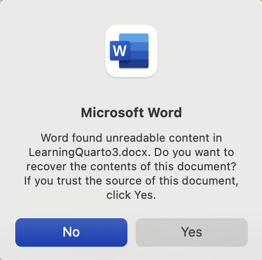
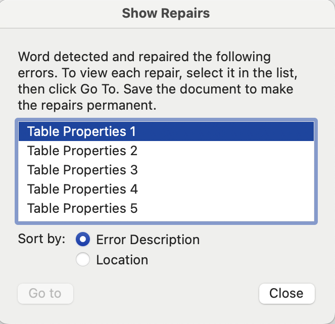
.docx version of a Quarto document.
To share your work with LibreOffice, OnlyOffice, and OpenOffice users, use the .odt rendering option. This will generate an OpenDocument — an open standard file format that can be opened in any text-processing software, including Microsoft Word.
---
format: odt
---
By default, the quality of the images and graphs in rendered .docx and .odt files is low. This is to keep the file size reasonable. High-quality images can be rendered by specifying the image definition in the YAML option. To do so, replace the format line that you added above with the following lines. Make sure that you indent each line correctly as shown below; otherwise, you will get an error when you try to render your document.
---
format:
  odt:
    fig-dpi: 300
---
TipYour turn!
Q14.15 If you completed Q8.15 (Section 8.3.1), you copied-and-pasted a paragraph with gaps into LibreOffice Writer or Microsoft Word and then manually inserted descriptive statistics that you had calculated in R. This method of copying-and-pasting across different programmes is very error-prone: What if you accidentally pasted the wrong number in the wrong place? And what if there was an update to the dataset or you made some changes to the data cleaning procedure? You’d have to manually change all the numbers again! 🤯 This is time-consuming and, more worryingly, very likely to result in errors!
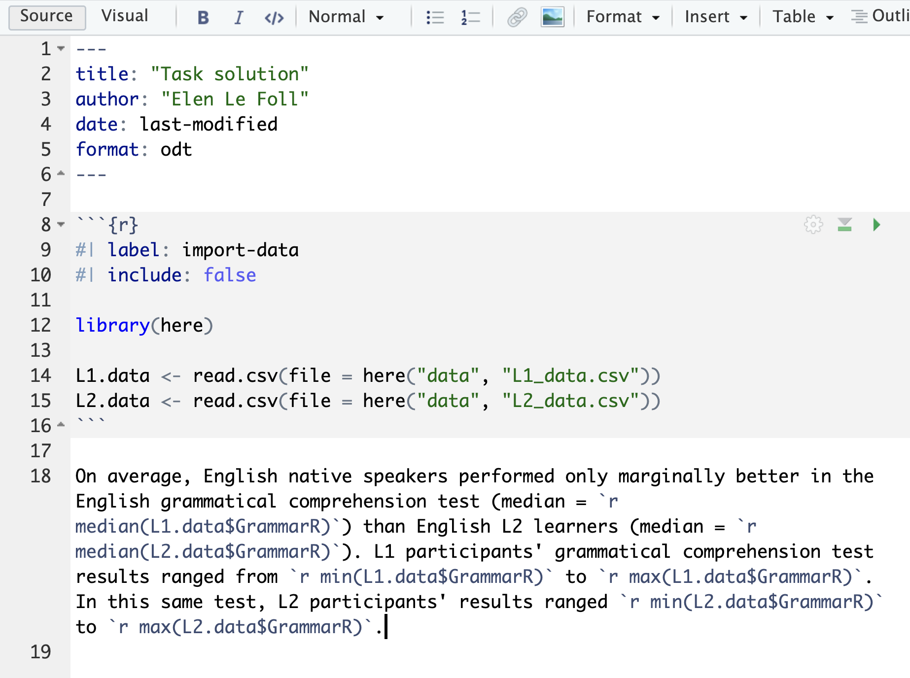
Now that you know about literate programming in Quarto, rewrite the following paragraph describing the GrammarR variable in L1.data and L2.data in Quarto. Use in-text code chunks to fill the gaps and then render your paragraph to .docx or .odt format to check the results.
On average, English native speakers performed only marginally better in the English grammatical comprehension test (median = ______) than English L2 learners (median = ______). However, L1 participants’ grammatical comprehension test results ranged from ______to ______, whereas L2 participants’ results ranged from ______to ______.
NoteClick here for the solution to Q14.15
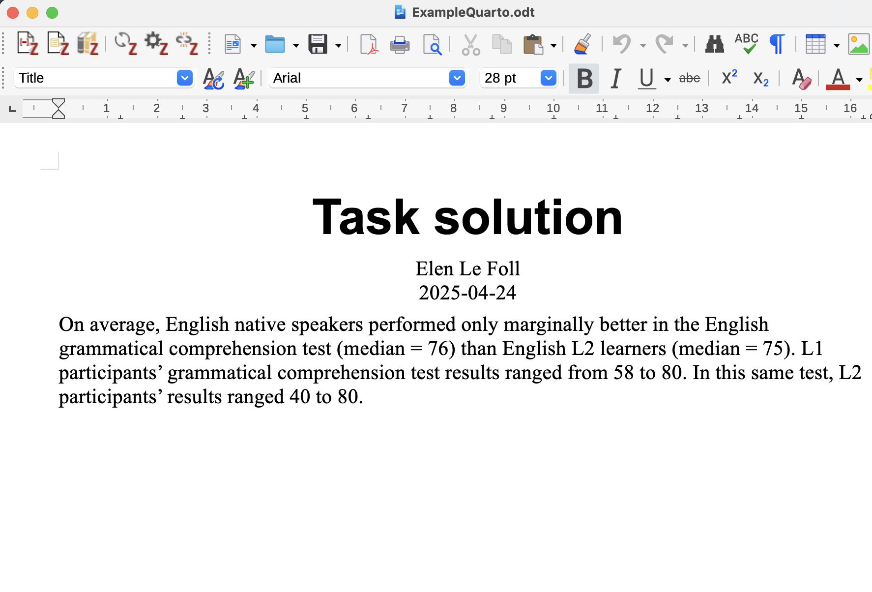
Below is a screenshot of a Quarto document with the inline code chunks and its rendered .odt version as opened in LibreOffice Writer. You can click on the images to zoom in.
14.13.2 PDF
It is also possible to render Quarto documents to PDF; however, this requires you to have LaTeX installed on your computer. Alternatively, you can use Typst — a new open-source markup-based typesetting system designed to be as powerful as LaTeX but easier to use.
If you don’t already have your favourite LaTex distribution, Quarto developers recommend that you use the TinyTeX distribution to render .qmd files to PDF. To install (or update) TinyTeX, go to the Terminal pane in RStudio and run the following command:
Terminal
quarto install tinytexThis is likely to take a few minutes but you will only need to do it once. Afterwards, you can add the following line to your Quarto YAML header and you’re ready to render to PDF! If you run into any issues installing {tinytex}, consult the tinytex FAQ page.
---
format: pdf
---
HTML being the default format, some options available for HTML are not – at least by default – available in other publishing formats. Many of the basic options, however, work across different formats. The YAML header options below can be used to include a table of content with numbered sections at the start of the PDF version of your document. It also includes two options that are specific to the PDF format and which are particularly useful for academic writing: the first will print a list of figures (lof) and the second a list of tables (lot).
---
format:
  pdf:
    number-sections: true
    toc: true
    lof: true
    lot: true
---
14.13.3 Slides
In research, it’s quite common that you will be working on a project that will be submitted as a paper or thesis (e.g. in PDF format) and that you’ll also want to present in class, to your research group, or at a conference. Conveniently, we can turn any Quarto document into presentation slides. At the time of writing, there are three presentation formats to choose from:
| Revealjs | An open-source HTML presentation framework. | format: revealjs |
| Power-Point | Microsoft Office’s presentation editing software. | format: pptx |
| Beamer | A LaTeX class for producing presentations and slides in PDF format. | format: beamer |
I recommend using Revealjs. The best way to get a sense of what is possible is to explore the demo presentation from the Quarto Guide.
14.14 Conclusion
This chapter only just scratched the surface of what’s possible in Quarto. The Quarto documentation is very detailed and well worth exploring to find out what else you can do in Quarto: https://quarto.org/docs/guide/. From books to blogs and interactive dashboards, the world’s your oyster! 🚀
NoteGoing further with Quarto
For those of you who want to dive a little deeper, I heartily recommend the final chapter of “An Introduction to Quantitative Text Analysis for Linguistics: Reproducible Research Using R” by Jerid Francom.
The latest edition of “R for Data Science” also has a great chapter on communicating the results of data science projects using Quarto.
Quarto for Scientists by Nicholas Tierney has many overlaps with this chapter but, as a “living book”, it is being regularly updated and expanded. The section on Common Problems with Quarto (and some solutions) is particularly useful.
Quarto has many functionalities that are particularly attractive to those of us involved in higher education teaching and academic research. Watch Quarto for Academics (20 minutes) by Mine Çetinkaya-Rundel to find out more.
Thinking of writing a term paper, thesis, dissertation, or book in Quarto? Cameron Patrick wrote his doctoral thesis in Quarto and has helpfully put together some great tips so that his “pain and suffering can help reduce yours”. Similarly, Gina Reinhard wrote her M.A. thesis as a single Quarto document and has made her Quarto template for term papers and theses available to all in open access.
Last but not least, Awesome Quarto provides a curated and regularly updated list of the many Quarto-related docs, talks, tools, examples, and articles that the internet has to offer.
Check your progress 🌟
Well done! You have successfully completed this chapter on literate programming using Quarto. You have answered 0 out of 16 questions correctly.
Are you confident that you can…?
Although there is ground for optimism here as more and more linguists and language education scholars are beginning to make their data open in repositories such as IRIS, TROLLing, and the Open Science Framework (OSF) (see Section 2.4).↩︎
The above definitions are all from the community-sourced FORRT glossary (Parsons et al. 2022).↩︎
Many other IDEs (Integrated Developer Environments, see Section 4.2.1) support Quarto, including JupyterLab, Neovim, Positron, and VS Code. Feel free to pick the IDE that you are most comfortable with!↩︎
If you need to install Quarto, go to https://quarto.org/docs/get-started/ and download the latest Quarto version that is compatible with your operating system. Once the download is completed (which may take several minutes), double-click on the installer file that you downloaded and click your way through the installation process.↩︎
Note that, in YAML syntax, character strings that include special characters (e.g.
') need to be enclosed in quotation marks.↩︎You can change this behaviour in your RStudio preferences under Tools > Global Options > R Markdown by selecting or unselecting the option: “Show output inline for all R Markdown documents”.↩︎
Using Microsoft Excel to open these
.csvfiles can corrupt the files and can happen even if you did not use Excel yourself (e.g. on some Windows computers, this is sometimes done automatically as part of the download process). To find out more, see Section 2.6.↩︎To make your Quarto document even more reproducible, you can replace your
setupchunk with the following function that will automatically check if a package needs to be installed before it is loaded:```{r} #| label: improved-setup # List of packages necessary in this Quarto document: packages <- c("here", "tidyverse", "xfun") # Function to install the packages that are not yet installed: installed_packages <- packages %in% rownames(installed.packages()) if (any(installed_packages == FALSE)) { install.packages(packages[!installed_packages], repos = "https://packagemanager.rstudio.com/all/latest") } # Function to load the packages without printing any messages: invisible(lapply(packages, library, character.only = TRUE)) ```To ensure that the correct package version is installed, consider using {renv} or {rix} for your project (see Section 14.10).↩︎