library(here)

Dabrowska.data <- readRDS(file = here("data", "processed", "combined_L1_L2_data.rds"))13 Multiple linear regRession modelling
Chapter overview
In this chapter, you will learn how to:
- Fit a linear regression model with multiple predictors
- Center numeric predictor variables when meaningful
- Interpret the coefficient estimates of a multiple linear regression model
- Interpret a model’s coefficients of determination (multiple R2 and adjusted R2)
- Compute and plot the relative importance of predictors
- Fit interaction effects and interpret their coefficient estimates
- Visualise the predictions of a multiple linear regression model and its (partial) residuals
- Report the results of a multiple linear regression model in tabular and graphical formats
- Check that the assumptions of multiple linear regression models are met.
13.1 From simple to multiple linear regression models
In Chapter 12, we used the lm() function to fit simple linear regression models. We saw that, like the t.test() and the cor.test() functions, the lm() function takes a formula as its first argument. Schematically, the formula syntax for a simple linear regression model takes the form of:
outcome.variable ~ predictorIn the second half of this chapter, we will continue to try to predict (i.e. try to better understand) Vocab scores among L1 and L2 English speakers, but this time, we will do so with multiple predictors. To this end, we will use the + operator to add predictors to our model formula like this:
outcome.variable ~ predictor1 + predictor2 + predictor3A linear regression model can include as many predictors as we like – or rather, as is meaningful and we have data for! The predictors can be a mixture of numeric and categorical predictors. Multiple linear regression modelling is much more powerful than conducting individual statistical tests (as in Chapter 11) or several simple linear regression models (as in Chapter 12) because it enables us to quantify the strength of the association between an outcome variable and a predictor, while controlling for the other predictors – in other words, while holding all the other predictors constant. Moreover, it also reduces the risk of reporting false positive results (i.e. Type 1 error, see Section 11.7). In this chapter, we will see that we can learn much more about our data from a single multiple linear regression model than from a series of individual statistical tests or simple regression models.
WarningPrerequisites
As with previous chapters, all the examples, tasks, and quiz questions from this chapter are based on data from:
Dąbrowska, Ewa. 2019. Experience, Aptitude, and Individual Differences in Linguistic Attainment: A Comparison of Native and Nonnative Speakers. Language Learning 69(S1). 72–100. https://doi.org/10.1111/lang.12323.
Our starting point for this chapter is the wrangled combined dataset that we created and saved in Chapter 9. Follow the instructions in Section 9.7 to create this R object.
Alternatively, you can download Dabrowska2019.zip from the textbook’s GitHub repository. To launch the project correctly, unzip the file and then double-click on the Dabrowska2019.Rproj file.
To begin, load the combined_L1_L2_data.rds file that we created in Chapter 9. This file contains the full data of all the L1 and L2 participants from Dąbrowska (2019). The categorical variables are stored as factors, and obvious data entry inconsistencies and typos have been corrected.
Before you get started, check that you have correctly imported the data by examining the output of View(Dabrowska.data) and str(Dabrowska.data). In addition, run the following lines of code to load the {tidyverse} and create “clean” versions of both the L1 and L2 datasets as separate R objects.
library(tidyverse)

L1.data <- Dabrowska.data |>
  filter(Group == "L1")

L2.data <- Dabrowska.data |>
  filter(Group == "L2")
Once you are satisfied that the data have been correctly imported and that you are familiar with the dataset, you are ready to tap into the potential of multiple linear regression modelling! 🚀
13.2 Combining multiple predictors
In the following, we will attempt to model the variability in the receptive English vocabulary test scores of L1 and L2 English participants from Dąbrowska (2019). To this end, we will use multiple numeric and categorical predictors:
- participants’ native-speaker status (
Group) - their
Age, - their occupational group (
OccupGroup), - their
Gender - their non-verbal IQ test score (
Blocks), and - the number of years they were in formal education (
EduTotal).
We use the + operator to construct the model formula. It doesn’t matter in which order we list the predictors, as the model will consider them all simultaneously.
model4 <- lm(Vocab ~ Group + Age + OccupGroup + Gender + Blocks + EduTotal,
             data = Dabrowska.data)
We can then examine the model summary just like we did in Chapter 12 using the summary() function:
summary(model4)
Call:
lm(formula = Vocab ~ Group + Age + OccupGroup + Gender + Blocks +
    EduTotal, data = Dabrowska.data)

Residuals:
    Min      1Q  Median      3Q     Max
-62.825 -10.838   1.831  12.185  38.345

Coefficients:
             Estimate Std. Error t value Pr(>|t|)
(Intercept)    4.2113    10.7831   0.391 0.696691
GroupL2      -22.2896     3.4854  -6.395 1.98e-09 ***
Age            0.3718     0.1401   2.654 0.008812 **
OccupGroupI    9.9519     5.5999   1.777 0.077600 .
OccupGroupM   -3.9993     4.5139  -0.886 0.377050
OccupGroupPS  -1.0629     4.3876  -0.242 0.808919
GenderM       -3.7177     3.1387  -1.184 0.238131
Blocks         1.3011     0.3218   4.043 8.44e-05 ***
EduTotal       2.4308     0.6293   3.863 0.000167 ***
---
Signif. codes:  0 '***' 0.001 '**' 0.01 '*' 0.05 '.' 0.1 ' ' 1

Residual standard error: 18.65 on 148 degrees of freedom
Multiple R-squared:  0.3621,    Adjusted R-squared:  0.3276
F-statistic:  10.5 on 8 and 148 DF,  p-value: 1.327e-11
As with the simple linear regression models, we begin our interpretation of the model summary with the coefficient estimate for the intercept (see Section 12.2). The first question we ask ourselves is:
- In this model, what does the intercept correspond to?
Remember that the reference levels of categorical predictors correspond to the first level of these variables. This is why, here, the coefficient estimate for the intercept corresponds to a female English native speaker with a clerical occupation:
levels(Dabrowska.data$Gender) # 'Female' is the first level.[1] "F" "M"levels(Dabrowska.data$Group) # 'L1' is the first level.[1] "L1" "L2"levels(Dabrowska.data$OccupGroup) # 'C' corresponding to a clerical professional occupation is the first level.[1] "C" "I" "M" "PS"The reference level of the numeric predictors, by contrast, corresponds to the value of zero. In model4, therefore, the estimated coefficient for the intercept corresponds to the predicted Vocab score of an adult English native speaker who belongs to the occupational group “C”, is female, who is aged 0 (!), scored 0 on the Blocks test, and spent 0 years (!) in formal education. Needless to say that trying to interpret this value is utterly meaningless! This is why, in this case, it makes sense to center our numeric predictor variables before entering them into our model. Another way to go about this would be to standardise the predictors using a z-transformation (see e.g. Winter 2019: Section 5.2).
13.3 Centering numeric predictors
Centering involves subtracting a variable’s average from each value in the variable. Typically, we subtract the mean from each value but, given that we saw that many of the numeric variables in our dataset are not at all normally distributed (see Section 8.2.2), here, we will subtract the median instead.
To this end, we use the mutate() function to add three columns to the R data object Dabrowska.data. These new columns contain transformed versions of the predictor variables that we previously entered into our model:
Dabrowska.data <- Dabrowska.data |>
  mutate(Age_c = Age - median(Age),
         Blocks_c = Blocks - median(Blocks),
         EduTotal_c = EduTotal - median(EduTotal))
We have centred the values of the three numeric predictor variables so that a value of zero in the transformed version corresponds to the variable’s original median value (see Table 13.1).
| Age | Age_c | Blocks | Blocks_c | EduTotal | EduTotal_c |
|---|---|---|---|---|---|
| 21 | -10 | 16 | 0 | 17 | 3 |
| 27 | -4 | 21 | 5 | 18 | 4 |
| 25 | -6 | 21 | 5 | 18 | 4 |
| 31 | 0 | 8 | -8 | 13 | -1 |
| 37 | 6 | 9 | -7 | 12 | -2 |
| 60 | 29 | 1 | -15 | 10 | -4 |
| 20 | -11 | 17 | 1 | 12 | -2 |
| 25 | -6 | 20 | 4 | 12 | -2 |
| 62 | 31 | 8 | -8 | 14 | 0 |
| 42 | 11 | 21 | 5 | 15 | 1 |
For each pair of variables, the value of 0 in the centered variable corresponds to the median value of the untransformed variable. As a result, in the centered variables, each data point is expressed in terms of how much it is either above the median (positive score) or below the median (negative score).
13.4 Interpreting a model summary
We can now fit a new multiple linear regression model that attempts to predict Vocab scores with the same predictors as model4 above, except that we are now entering the centered numeric predictor variables instead of the original untransformed ones. The categorical predictor variables remain the same.
model4_c <- lm(Vocab ~ Group + Age_c + OccupGroup + Gender + Blocks_c + EduTotal_c,
             data = Dabrowska.data)

summary(model4_c)
Call:
lm(formula = Vocab ~ Group + Age_c + OccupGroup + Gender + Blocks_c +
    EduTotal_c, data = Dabrowska.data)

Residuals:
    Min      1Q  Median      3Q     Max
-62.825 -10.838   1.831  12.185  38.345

Coefficients:
             Estimate Std. Error t value Pr(>|t|)
(Intercept)   70.5852     3.7045  19.054  < 2e-16 ***
GroupL2      -22.2896     3.4854  -6.395 1.98e-09 ***
Age_c          0.3718     0.1401   2.654 0.008812 **
OccupGroupI    9.9519     5.5999   1.777 0.077600 .
OccupGroupM   -3.9993     4.5139  -0.886 0.377050
OccupGroupPS  -1.0629     4.3876  -0.242 0.808919
GenderM       -3.7177     3.1387  -1.184 0.238131
Blocks_c       1.3011     0.3218   4.043 8.44e-05 ***
EduTotal_c     2.4308     0.6293   3.863 0.000167 ***
---
Signif. codes:  0 '***' 0.001 '**' 0.01 '*' 0.05 '.' 0.1 ' ' 1

Residual standard error: 18.65 on 148 degrees of freedom
Multiple R-squared:  0.3621,    Adjusted R-squared:  0.3276
F-statistic:  10.5 on 8 and 148 DF,  p-value: 1.327e-11
If you compare the summary of model4 with that of model4_c, you will notice that, whilst the intercept coefficient estimate has changed, all the other coefficient estimates have stayed the same.
Let’s decipher the summary of model4_c step-by-step:
In this model, the estimated coefficient for the intercept corresponds to the predicted
Vocabscore of an English native speaker (Group= L1) who is aged 31 (the medianAge), belongs to the occupational groupC, is female, scored 16 on the Blocks test (the medianBlocksscore), and was in formal education for 14 years (the median number of years).As with the simple linear regression models that we computed in Chapter 12, the coefficient estimates of the numeric predictors (
Age_c,Blocks_c, andEduTotal_c) correspond to increases or decreases inVocabscores for each additional unit of that predictor variable, whilst keeping all other predictors at their reference level. Remember that, for numeric predictors, the reference level is 0, which, given that we have centered them, corresponds to the variable’s median value. Looking at the coefficient estimate forBlocks_c(1.3011), this means that someone who scored one point more than the median score in the Blocks test is predicted to have aVocabtest result that is1.3011points higher than the intercept, namely:70.5852 + 1.3011[1] 71.8863To calculate the predicted
Vocabscore of an L1 female speaker in a clerical occupation, of median age, who spent the median number of years in formal education, but scored an impressive 26 points on the Blocks test, we multiply the estimatedBlocks_ccoefficient (1.3011) by 26 minus the median Blocks score (16) and add this to the intercept coefficient:70.5852 + 1.3011*(26 - median(Dabrowska.data$Blocks))[1] 83.5962You’ll be pleased to read that the interpretation of coefficient estimates of categorical predictors is less involved. Recall that, for categorical variables, the reference level is always the variable’s first level (see Section 13.2). If we want to make a prediction for an L2 instead of an L1 female speaker, but keep all other predictors at the reference level (i.e. clerical occupation, median age, median number of years in formal education, and median Blocks score), all we need to do is add the coefficient estimate for
GroupL2(-22.2896) to the intercept coefficient. Given that this coefficient is negative, this addition will result in a predictedVocabscore that is lower than the model’s reference level:70.5852 + -22.2896[1] 48.2956Since very few people are perfectly average, let us now calculate the predicted
Vocabscore of an actual, randomly chosen person: the 154th participant in our dataset. As shown below using the {tidyverse} functionslice(), the 154th participant is a 46-year-old Polish male driver who scored 23 points on the Blocks test and attended formal education for 10 years.Dabrowska.data |> slice(154) |> select(Group, Age, NativeLg, Occupation, OccupGroup, Gender, Blocks, EduTotal)Group Age NativeLg Occupation OccupGroup Gender Blocks EduTotal 1 L2 46 Polish Driver M M 23 10To obtain the model’s predicted
Vocabscore for a 46-year-old male L2 speaker with a manual occupation (M) who scored 23 points on theBlockstest and was in formal education for 10 years (EduTotal), we combine the coefficient estimates as follows:70.5852 + -22.2896 + 0.3718 * (46 - median(Dabrowska.data$Age)) + -3.9993 + -3.7177 + 1.3011 * (23 - median(Dabrowska.data$Blocks)) + 2.4308 * (10 - median(Dabrowska.data$EduTotal))- 1
- Intercept coefficient
- 2
- L2 speaker
- 3
- 46 years old
- 4
- Manual occupation (OccupGroupM)
- 5
- Male
- 6
- 23 points on Blocks test
- 7
- 10 years in formal education
[1] 45.5401TipYou can hover your mouse over the circled numbers to find out how this predicted score was calculated. All the coefficient estimates were copied from the model summary output by
summary(model4_c).We can check that we did the maths correctly by outputting the model’s prediction for the 154th observation directly. To this end, we apply the
predict()function to the model objectmodel4_cand extract the model’s predicted score for the 154th data point:predict(model4_c)[154]154 45.53989As you can see, we obtain the same predicted
Vocabscore. The minor difference after the decimal point is due to us using coefficient estimates rounded-off to four decimal places (as displayed in the model’s summary output) rather than the exact values to which thepredict()function has access.This is all very well, but how accurate is this model prediction? To find out, we can compare this predicted score (that our model predicts for any male 46-year old with a manual occupation, a Blocks score of 23, and 10 years in formal education) to the 46-year-old Polish driver’s actual
Vocabscore:Dabrowska.data |> slice(154) |> select(Group, Age, NativeLg, Occupation, OccupGroup, Gender, Blocks, EduTotal, Vocab)Group Age NativeLg Occupation OccupGroup Gender Blocks EduTotal Vocab 1 L2 46 Polish Driver M M 23 10 48.88889Our model prediction (
45.53989) is close to our Polish driver’s realVocabtest score (48.88889), but our model has slightly underestimated his performance. This underestimation results in a positive residual. The residual is positive because there are points “left over” by the model. Model residuals are calculated by subtracting a model’s prediction from the real, observed value of the outcome variable for any specific data point. In our case, we substract our model’s predictedVocabscore for a male 46-year old with a manual occupation, a Blocks score of 23, and 10 years in formal education from the Polish 46-year-old driver’s actualVocabscore:48.88889 - 45.53989[1] 3.349Residuals are also stored in the model object and be accesssed like this:
model4_c$residuals[154]154 3.348998We can compare this particular residual (corresponding to the 154th participant in the dataset) to all model residuals (corresponding to all participants) by examining the summary statistics of all residuals, which are displayed at the top of the model summary output (
summary(model4_c)). These descriptive statistics inform us that the residual for the 154th participant is slightly higher than the average (median) residual, but well within the IQR (see Section 8.3.2) of model residuals:Residuals: Min 1Q Median 3Q Max -62.825 -10.838 1.831 12.185 38.345Looking at the minimum and maximum residuals, we can see that our model overestimates at least one person’s
Vocabscore by 63 points (this is the most negative residual:Min), whilst in another case it underestimates it by 38 points (this is the largest positive residual:Max).Click here to find out whose score was most underestimated!
# Run the following code to find out more about the participant whose Vocab score was most dramatically underestimated by our model:

Dabrowska.data |>
  slice(which.max(model4_c$residuals)) |>
  select(Group, NativeLg, Age, Occupation, Gender, Blocks, EduTotal, Vocab)
The p-values associated with each coefficient estimate in the model summary indicate which predictor variables (or predictor variable levels, in the case of categorical variables) make a statistically significant contribution to the model. You may recall that, in Section 12.3, we fitted a simple linear regression model (
model3) which included onlyOccupGroupas a single predictor. In this simple model, the coefficient estimate forOccupGroupImade a statistically significant contribution to the model at an α-level of 0.05 (p = 0.0335). By contrast, in the present multiple linear regression model, the predictor levelOccupGroupIdoes not make a statistically significant contribution (p = 0.077600 which is greater than 0.05). This is because our multiple regression modelmodel4_cincludes predictors that account for some of the same variance inVocabscores in the data that occupational groups accounted for in our earlier model. This leaves less unique variance attributable to occupational group, thereby rendering it statistically non-significant.From the adjusted R-squared value (
0.3276) displayed at the bottom of the model summary output, we can see that our multiple linear regression model accounts for around 33% of the total variance inVocabscores found in the Dąbrowska (2019) data. This is considerably more than we achieved with any of the simple linear models that we fitted in Chapter 12.
13.4.1 Interpreting model predictions
Whilst it is important to understand how to interpret the coefficients of a multiple linear regression model from the model summary, in practice, it is also always a very good idea to visualise model predictions. On the one hand, this reduces the risk of making any obvious interpretation errors and, on the other, it is much easier to interpret the residuals of a model when they are visualised alongside model predictions.
To fully visualise the predictions of a multiple linear model, we would need to be able to plot as many dimensions as there are predictors in the model. The trouble is that, as humans, we find it difficult to interpret data visualisations with more than two dimensions. Indeed, although 3D plots can sometimes be useful (and can easily be generated in R), we are much better at interpreting two-dimensional plots. To bypass this inherent human weakness, we will plot the values predicted by our model on several plots: one for each predictor variable (see Figure 13.1). Run the following command and then follow the instructions displayed in the Console pane to view the plots one by one. You may need to resize your Plot pane for the plots to be displayed. If you have a small screen, you may find the “:magnifying-glass-tilted-right: Zoom” option in RStudio’s Plots pane useful as it allows you to view the plots in a separate window.
library(visreg)
visreg(model4_c)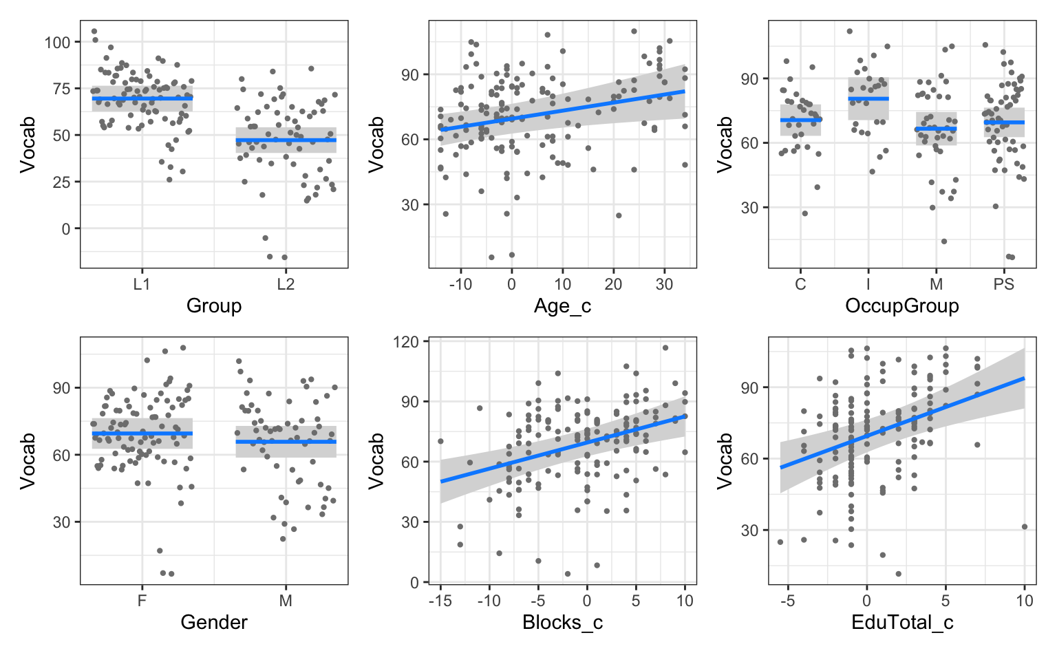
Vocab scores as predicted by model4_c (blue lines) as a function of various predictor variables and partial model residuals (grey points)
On plots produced by the visreg() function, as in Figure 12.9, the model’s predicted values are displayed as blue lines. By default, these predictions are surrounded by 95% confidence bands, which are visualised as grey areas. Now that we have several predictors in our model, the points in visreg() plots represent the model’s partial residuals. Partial residuals are the left-over variance (i.e. the residual) relative to the predictor that we are examining after having subtracted off the contribution of all the other predictors in the model.
When interpreting the numeric predictors plotted in Figure 13.1 above, it is important to remember that we entered centered numeric predictors in model4_c. This means that an Age_c value of 0 corresponds to the median age in the dataset: 31 years. This is why Figure 13.1 features negative ages: the negative values correspond to participants who are younger than 31. By contrast, positive scores correspond to participants who are older than 31 years. This is hardly intuitive so, for the purposes of visualising and interpreting our model, it is best to transform these variables back to their original scale (see Figure 13.2). This is achieved by adding the following xtrans argument within the visreg() function.
Warning
Due to a bug that was introduced in the latest version of the {visreg} package, it is currently necessary to install version 2.7 of the {visreg} package for the xtrans argument to work as expected. You can find out which package version you currently have installed, if any, using this function:
packageVersion("visreg")If you have version 2.8.0, begin by deleting your current installation:
remove.packages("visreg")Then, install the {remotes} package, which allows you to install older versions of packages (if they are compatible with your R version). You will likely get a message notifying you that it is necessary to restart your R session. Click “yes”.
install.packages("remotes")Finally, load the {remotes} library and then install version 2.7.0 of the {visreg} package:
library(remotes)
install_version("visreg", "2.7.0")library(visreg)
visreg(model4_c,
xvar = "Age_c",
xtrans = function(x) x + median(Dabrowska.data$Age),
gg = TRUE) +
labs(x = "Age (in years)",
y = "Predicted Vocab scores") +
theme_bw()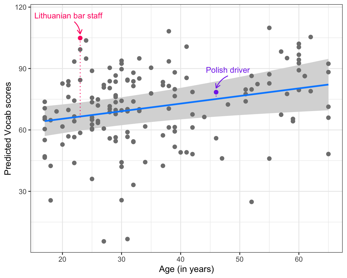
Vocab scores as predicted by model4_c for speakers of various ages (blue line) and partial model residuals represented as points. In the version printed in the textbook, two data points are highlighted: one representing a very large positive residual and one representing a very small residual.
In Figure 13.2, we focus on one predictor from our model: Age. We know from our model summary that the coefficient estimate for age is positive (0.3718), hence the upward blue line. The grey 95% confidence band visualises the uncertainty around the estimated mean predicted Vocab scores.
The points on Figure 13.2 represent the partial residuals. This means that there are as many points as there are participants in the dataset used to fit the model. The further away a point is from the predicted value (the blue line), the poorer the prediction is for that particular participant.
Some of the partial residuals are particularly large: the Vocab score of the 23-year-old Lithuanian bar staff, for instance, is vastly underestimated. By contrast, the 46-year-old Polish driver’s predicted score is well within the confidence band of the predicted Vocab score for his age, indicating that our model makes a pretty accurate prediction for this L2 speaker.
TipYour turn!
The dataset from Dąbrowska (2019) includes a variable that we have not explored yet: ART. It stands for Author Recognition Test (Acheson, Wells & MacDonald 2008) and is a measure of print exposure to (almost exclusively Western, English-language) literature. Dąbrowska (2019: 9) explains the testing instrument and her motivation for including it in her battery of tests as follows:
The test consists of a list of 130 names, half of which are names of real authors. The participants’ task is to mark the names that they know to be those of published authors. To penalize guessing, the score is computed by subtracting the number of foils [wrong guesses] from the number of real authors selected. Thus, the maximum possible score is 65, and the minimum score could be negative if a participant selects more foils than real authors. When this happened, the negative number was replaced with 0.
The ART has been shown to be a valid and reliable measure of print exposure, which, unlike questionnaire-based measures, is not contaminated by socially desirable responses and assesses lifetime reading experience as opposed to current reading (see Acheson et al., 2008; Stanovich & Cunningham, 1992).
Q13.1 For this task, you will fit a new multiple linear regression model that predicts Vocab scores among L1 and L2 speakers using all of the predictors that we used in model4_c plus ART scores. Which formula do you need to specify inside the lm()function to fit this new model (which we will name model.ART)?
🐭 Click on the mouse for a hint.
Q13.2 Fit a model using the correct formula from above and save it as model.ART. Examine the summary of your new model. Which of these statements is/are true?
🐭 Click on the mouse for a hint.
Show sample code to answer Q13.2.
# First, it is always a good idea to visualise the data before fitting a model to have an idea of what to expect:
Dabrowska.data |>
ggplot(mapping = aes(y = Vocab,
x = ART)) +
geom_point() +
geom_smooth(method = "lm") +
theme_bw()
# We fit the new model with ART as an additional predictor using the formula from Q13.1:
model.ART <- lm(Vocab ~ Group + Age_c + OccupGroup + Gender + Blocks_c + EduTotal_c + ART,
data = Dabrowska.data)
# We examine the coefficients of this new model:
summary(model.ART)
# To find out how much variance the model accounts for compared to our prior model, compare the adjusted R-squared values of the two models:
summary(model4_c)
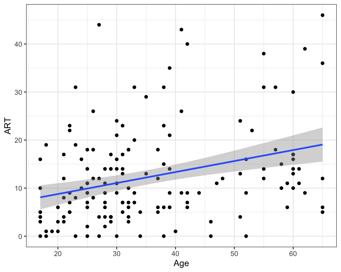
summary(model.ART)Have you noticed how, having added ART as a predictor to your model, Age no longer makes a statistically significant contribution to the model (p = 0.070994)? How come? Well, it turns out that ART and Age are correlated (r = 0.32, see scatter plot below). This moderate positive correlation makes intuitive sense: the older you are, the more likely you are to have come across more authors and therefore be able to correctly identify them in the Author Recognition Test. Of the two predictors, our model suggests that ART scores are a more useful predictor of Vocab scores than age. In other words, if we know the ART score of a participant from the Dąbrowska (2019) dataset, their age does not provide additional information that can help us to better predict their Vocab score.
Q13.3 What is the predicted Vocab score of a female L1 speaker aged 31 (the median age) with a manual occupation, who scored 16 on the Blocks test (the median score), spent 14 years in formal education (median time period), and scored 20 on the Author Recognition Test?
🐭 Click on the mouse for a hint.
Show sample code to answer Q13.3.
# We must add together the coefficient for the intercept, the coefficient for the manual occupation (which is negative), and the ART coefficient multiplied by 20 (as we did not center this predictor):
62.5728 + -2.5115 + 0.5526*20
Q13.4 By default, the visreg() function displays a 95% confidence band around predicted values, corresponding to a significance level of 0.05. How can you change this default to display a 99% confidence band instead? Run the command ?visreg() to find out how to achieve this from the function’s help file.
🐭 Click on the mouse for a hint.
Show sample code to answer Q13.4.
# The argument that you need to change is called "alpha". This is because the significance level is also called the alpha level (see Section 11.3).

# The alpha value that corresponds to a 99% confidence interval is equal to:
1 - 0.99

# Hence the code should (minimally) include these arguments:
visreg(model.ART,
       xvar = "ART",
       alpha = .01)
Observe how the width of the confidence bands changes when you increase the significance level from 0.01 to 0.1: the higher the significance level, the narrower the confidence band becomes. Remember that the significance level corresponds to the risk that we are willing to take of wrongly rejecting the null hypothesis when it is actually true. Therefore, when we lower this risk by choosing a lower significance level (i.e. 0.01), we end up with wider confidence bands that are more likely to allow us to draw a flat line (see Section 11.5). If we can draw a flat line through a 99% confidence band, this means that we do not have enough evidence to reject the null hypothesis at the significance level of 0.01.
13.5 Relative importance of predictors
When interpreting a model summary, it is important to remember that the coefficient estimates of each predictor correspond to a change in prediction for a one-unit change in that predictor, e.g. for the predictor Age, an increase of one year. However, within a single model, it’s quite common for the predictor variables to be measured in different units. For example, in summary(model4_c), the coefficient estimate for Age_c is 0.3718, which means that, holding all other predictors constant, for every year that a participant is older than the median age, their predicted Vocab score increases by 0.3718. By contrast, the coefficient estimate for the Blocks_c predictor (1.3011) corresponds to an increase in Vocab scores for every additional point that participants score on the non-verbal IQ Blocks test. Its unit is therefore test points. For categorical predictor variables, a single-unit change represents a change from one predictor level to another, e.g. from L1 to L2, or from female to male.
Because they are in different units that represent different quantities or levels, the raw coefficient estimates of a model cannot be compared to each other. Indeed, depending on the predictor, a one-unit change may correspond to either a big or a small change. This is where measures of the relative importance of predictors come in handy. In this chapter, we will use the lmg metric (that was first proposed by Lindeman, Merenda & Gold in 1980: 119 ff.) to compare the importance of predictors within a single multiple linear regression model.
Although not currently widely used in the language sciences (but see, e.g. Dąbrowska 2019: 14), lmg has a number of advantages. Its interpretation is fairly intuitive because it is similar to a coefficient of determination (R2): a value of 0 means that, in this model, a predictor accounts for 0% of the variance in the outcome variable, while a value of 1 would mean that it can be used to perfectly predict the outcome variable. Calculating lmg values is computationally involved because the metric includes both direct effects and is adjusted for all the other predictors of the model. But this need not worry us because a researcher and statistician, Ulrike Grömping, has developed and published an R package that will do the computation for us. :smiling-face-with-smiling-eyes:
Once we have installed and loaded the {relaimpo} package1 (Grömping 2006), we can use its calc.relimp() function to calculate a range of relative importance metrics for linear models. With the argument “type”, we specify that we are interested in the lmg metric:
install.packages("relaimpo")
library(relaimpo)
select <- dplyr::select

rel.imp.metric <- calc.relimp(model4_c,
                              type = "lmg")
The output of the function is long. We have therefore saved it as a new R object (rel.imp.metric) in order to retrieve only the part that we are interested in, namely the lmp values for each predictor, as a single data frame (rel.imp.metric.df):
rel.imp.metric.df <- data.frame(lmg = rel.imp.metric$lmg) |>
    rownames_to_column(var = "Predictor")
We display this data frame in descending order of lmp values, rounded to two decimal values:
rel.imp.metric.df |>
  mutate(lmg = round(lmg, digits = 2)) |>
  arrange(-lmg)
Predictor lmg
1 Group 0.15
2 OccupGroup 0.07
3 EduTotal_c 0.05
4 Age_c 0.04
5 Blocks_c 0.04
6 Gender 0.00These values indicate that, on average, whether or not a participant is a native or non-native speaker of English (Group) makes the biggest difference in terms of predicted Vocab scores. Gender, by contrast, is practically irrelevant in this model.
We can also visualise these values in the form of a bar plot (see Figure 13.3). Note that another nice thing about the lmg metric is that the lmg values for all the predictors entered in model4_c add up to the model’s (unadjusted) multiple R2 (0.3621).
rel.imp.metric.df |>
  ggplot(mapping = aes(x = fct_reorder(Predictor, lmg),
                       y = lmg)) +
  geom_col() +
  theme_minimal() +
  labs(x = "Predictor in model4_c") +
coord_flip() 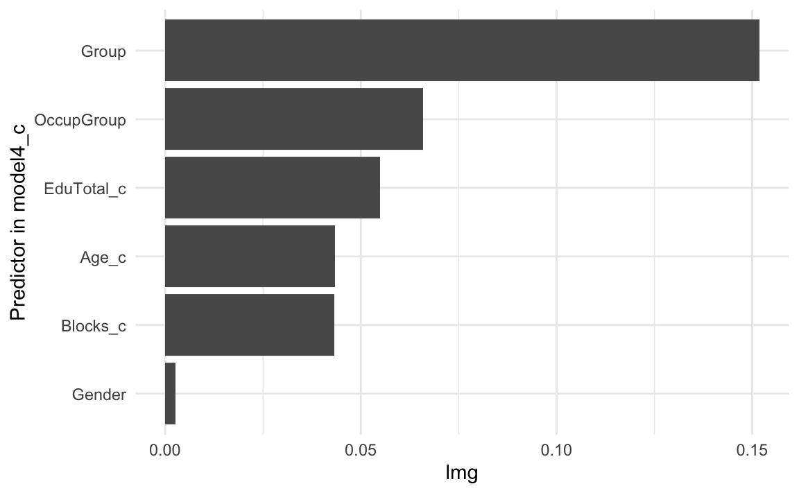
model 4_c
It is also worth noting that the second most important predictor is OccupGroup. This may come as a surprise given that none of its levels (or rather none of the differences between the reference level of C for clerical occupations and the remaining levels) make a statistically significant contribution to the model. This result illustrates the value of this type of analysis compared to only looking at a model’s coefficient estimates.
Many studies will compare the coefficient estimates of multiple regression models using standardised coefficients (see e.g. Winter 2019: Section 6.2); however, this approach can lead to misleading conclusions (see e.g. Mizumoto 2023).
TipYour turn!
In the last Your turn! section, you fitted a multiple linear regression model to predict Vocab scores among L1 and L2 speakers using all of the predictors that we used in model4_c plus ART scores.
Q13.5 Calculate the relative importance of each of the predictors in this model using the {relaimpo} package. What is the relative importance of the predictor ART in this model as estimated by the lmg metric and rounded to two decimal places?
Show sample code to answer Q13.5.
# Fit the model:
model.ART <- lm(Vocab ~ Group + Age_c + OccupGroup + Gender + Blocks_c + EduTotal_c + ART,
             data = Dabrowska.data)

# Compute the lmg values and extract them as a data frame
library(relaimpo)
rel.imp.metric <- calc.relimp(model.ART,
                              type = "lmg")

rel.imp.metric.df <- data.frame(lmg = rel.imp.metric$lmg) |>
    rownames_to_column(var = "Predictor")

rel.imp.metric.df |>
  mutate(lmg = round(lmg, digits = 2)) |>
  arrange(-lmg)
13.6 Modelling interactions between predictors
One of the strengths of multiple linear regression is that we can also model interactions between predictors. This is important because a predictor’s relationship with the outcome variable may depend on another predictor. Consider Age as a predictor of Vocab scores. In model4_c, we saw that this predictor made a statistically significant contribution to the model. The coefficient was positive, which means that the model predicts that the older the participants, the higher their receptive English vocabulary.
However, if you completed Q11.10, you might remember that Age correlates positively with Vocab scores among L1 participants, but does not among L2 participants (see Figure 13.4 below). If anything, the correlation visualised in the right-hand panel of Figure 13.4 is slightly negative. Moreover, the confidence band is wide enough to draw a horizontal line through it, which suggests that the data are also compatible with the null hypothesis of no correlation. As a result, we can conclude that this slightly negative correlation is not statistically significant.
Dabrowska.data |>
   ggplot(mapping = aes(x = Age,
                        y = Vocab)) +
     geom_point() +
     facet_wrap(~ Group) +
     geom_smooth(method = "lm",
                 se = TRUE) +
  theme_bw()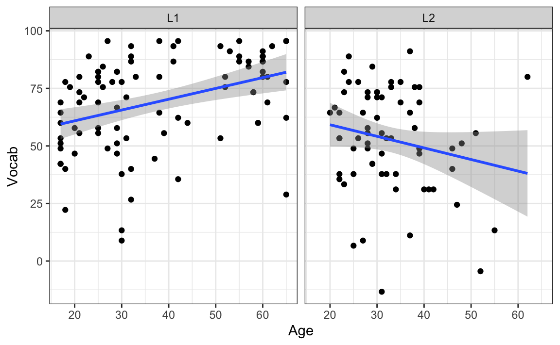
Figure 13.4 informs us that what we really need is a model that can account for the fact that Age is probably a useful predictor of Vocab scores for L1 speakers, but not so much for L2 speakers. In other words, we’d like to model an interaction between the predictors Age and Group.
In R’s formula syntax, interaction terms are denoted with a colon (:) or an asterisk (*). In the following model, therefore, we are attempting to predict Vocab scores on the basis of a person’s native-speaker status (Group), their age, occupational group, gender, Blocks test score, number of years in formal education, and the interaction between their age and native-speaker status (Age_c:Group):
model5 <- lm(Vocab ~ Group + Age_c + OccupGroup + Gender + Blocks_c + EduTotal_c + Age_c:Group,
             data = Dabrowska.data)

summary(model5)
Call:
lm(formula = Vocab ~ Group + Age_c + OccupGroup + Gender + Blocks_c +
    EduTotal_c + Age_c:Group, data = Dabrowska.data)

Residuals:
    Min      1Q  Median      3Q     Max
-66.720 -10.651   1.224  11.939  45.415

Coefficients:
              Estimate Std. Error t value Pr(>|t|)
(Intercept)    69.1314     3.6286  19.052  < 2e-16 ***
GroupL2       -19.9128     3.4699  -5.739 5.26e-08 ***
Age_c           0.5466     0.1471   3.717 0.000286 ***
OccupGroupI     7.8267     5.4824   1.428 0.155525
OccupGroupM    -4.0769     4.3852  -0.930 0.354058
OccupGroupPS   -1.7774     4.2686  -0.416 0.677729
GenderM        -1.6285     3.1213  -0.522 0.602644
Blocks_c        1.2414     0.3132   3.964 0.000115 ***
EduTotal_c      2.5520     0.6126   4.166 5.27e-05 ***
GroupL2:Age_c  -0.8982     0.2867  -3.133 0.002089 **
---
Signif. codes:  0 '***' 0.001 '**' 0.01 '*' 0.05 '.' 0.1 ' ' 1

Residual standard error: 18.12 on 147 degrees of freedom
Multiple R-squared:  0.402, Adjusted R-squared:  0.3654
F-statistic: 10.98 on 9 and 147 DF,  p-value: 5.537e-13
In the model summary above, the interaction term between Age and Group is the last coefficient listed (GroupL2:Age_c). The values confirm our intuition based on our descriptive visualisation of the data (Figure 13.4): there is a statistically significant interaction between age and native-speaker status (p = 0.002089) and the interaction coefficient for this interaction term (Age_c:Group) is negative (-0.8982). This means that, whilst being older is generally associated with higher Vocab scores for the reference level of L1 speakers, if a participant is an L2 English speaker, this trend is reversed.
To understand how this works in practice, let’s compare the predicted Vocab scores of two 35-year-olds: one a native English speaker and the other a non-native. For the purposes of this illustration, we will assume that, apart from their native-speaker status, all their other characteristics correspond to the reference level in our model (i.e. they are both female, have a clerical occupation, scored average on the Blocks test and were in formal education for the median number of years). For the L1 speaker, we calculate their predicted Vocab score as before. We take the intercept (69.1314) as our starting point and then add the Age_c coefficient (0.5466) multiplied by the difference between their age and the median age (which is the reference level of our centered predictor) (i.e. 35 - 31 = 4). This means that their predicted Vocab score is:
69.1314 + 0.5466*4[1] 71.3178For the L2 speaker, we begin by combining the same coefficient estimates as above but, this time, we also add the GroupL2 coefficient (-19.9128), and the interaction coefficient (GroupL2:Age_c). The interaction coefficient (-0.8982) has to be multiplied by the difference between the speaker’s age and the median age (which remains 4 years). This L2 speaker’s predicted score is therefore:
69.1314 + 0.5466*4 + -19.9128 + -0.8982*4[1] 47.8122
CautionImportant
Whenever we have a model with an interaction, we can no longer interpret the individual coefficient estimates of the predictors that enter into the interaction by themselves: instead, we must interpret our model’s main effects together with their interaction!
For example, in model5, if we only took account of the model’s main effect for age, we would be misled into thinking that age is always positively associated with Vocab scores. However, as illustrated in Figure 13.4, we know that this is not true for L2 speakers — hence the statistically significant interaction between Age_c and Group in model5.
The best way to avoid misinterpreting interaction effects is to make sure you always visualise the predictions of models that involve interactions. The visreg() function includes a “by” argument, which is ideal for this:
visreg(model5,
       xvar = "Age_c",
       by = "Group",
       xtrans = function(x) x + median(Dabrowska.data$Age),
       gg = TRUE) +
  labs(x = "Age (in years)",
       y = "Predicted Vocab scores") +
  theme_bw()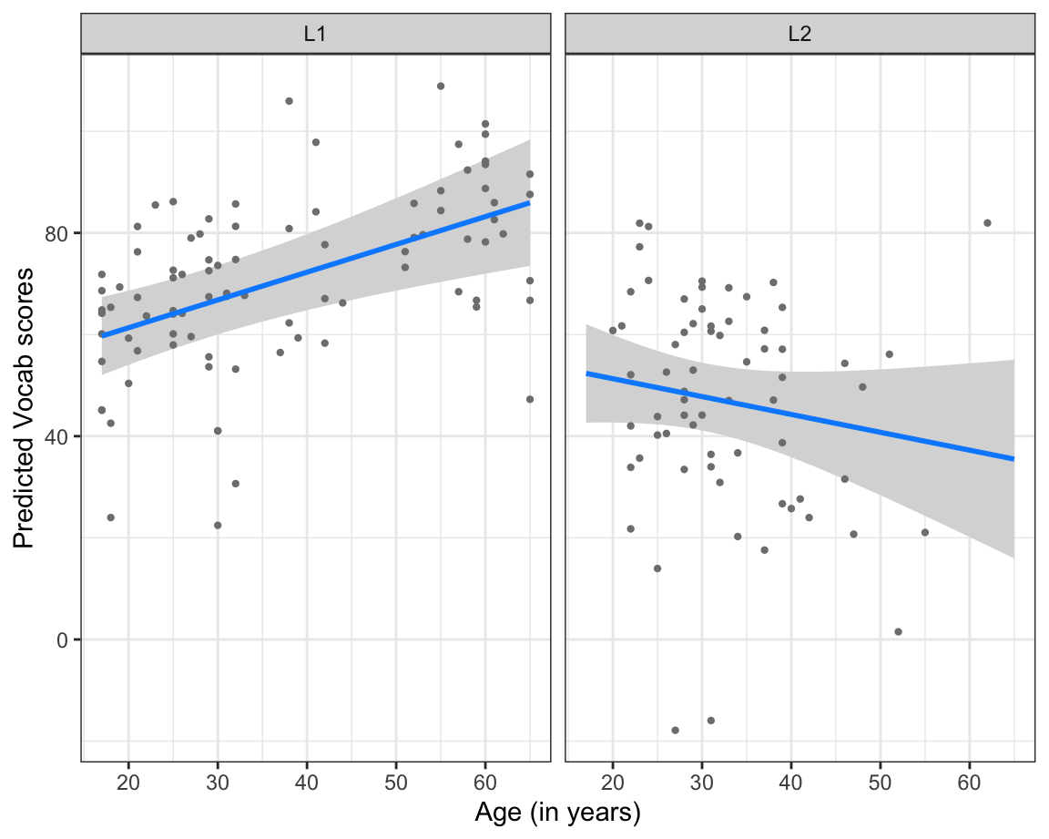
Vocab scores as predicted by model5 for L1 and L2 speakers of various ages (blue lines) and partial model residuals (grey points)
If we compare Figure 13.5 (in which the points represent the model’s partial residuals) to Figure 13.4 (in which the points represent the actual, observed values), we can see that the partial residuals are, on average, smaller than the differences between the observed values and the regression lines of Figure 13.4. This is because the regression lines of Figure 13.4 correspond to a model that only includes three coefficients, Age_c, Group and their interaction (Age_c:Group), whereas the partial residuals in Figure 13.5 correspond to the left-over variance in Vocab scores once all other predictors of the model5 have been taken into account.
Comparing the model summaries of model4_c and model5, we can see that adding the interaction term between age and native-speaker status considerably boosted the amount of variance in Vocab scores that our model now accounts for: whereas the adjusted R2 of the model without the interaction was 0.3276 (33%), it has now reached 0.3654 (37%) thanks to the added interaction.
TipYour turn!
In this task, we will explore the possibility of an interaction between participants’ native-speaker status (Group) and the number of years they spent in formal education (EduTotal). The underlying idea is that, for the L1 speakers, their formal education will most likely have been in English; hence the longer they were in formal education, the higher they might score on the Vocab test. For the L2 speakers, however, their formal education will more likely have been in a language other than English. As a result, years in formal education may be a weaker predictor of Vocab scores than for L1 speakers.
Q13.6 To begin, generate a plot to visualise this interaction in the observed data: map the EduTotal variable onto the x-axis and Vocab onto the y-axis, and split the plot into two facets, one for L1 and the other for L2 participants. Based on your interpretation of your plot, which of these statements is/are correct?
🐭 Click on the mouse for a hint.
Show code to generate the plot needed to complete Q13.6
Dabrowska.data |>
   ggplot(mapping = aes(x = EduTotal,
                        y = Vocab)) +
     geom_point() +
     facet_wrap(~ Group) +
     geom_smooth(method = "lm",
                 se = TRUE) +
     theme_bw()
Q13.7 Below is the model formula for model5:
Vocab ~ Group + Age_c + OccupGroup + Gender + Blocks_c + EduTotal_c + Age_c:GroupWhat do you need to add to this formula to also model the interaction that you just visualised?
Q13.8 Fit the model with the added interaction. Does the interaction make a statistically significant contribution to the model at the significance level of 0.05?
Show code to complete Q13.8
model5.int <- lm(Vocab ~ Group + Age_c + OccupGroup + Gender + Blocks_c + EduTotal_c + Age_c:Group + EduTotal_c:Group,
                 data = Dabrowska.data)

summary(model5.int)
Q13.9 Use the {visreg} package to visualise the interaction effect EduTotal_c:Group as predicted by your model. Looking at your plot of predicted values and partial residuals, which conclusion can you draw?
🐭 Click on the mouse for a hint.
Show code to help you complete Q13.9
visreg(model5.int,
       xvar = "EduTotal_c",
       by = "Group",
       xtrans = function(x) x + median(Dabrowska.data$EduTotal),
       gg = TRUE) +
  labs(x = "Years in formal education",
       y = "Predicted Vocab scores") +
  theme_bw()
13.6.1 Interactions between two numeric predictors
We can also model interactions between two numeric predictors. For instance, we may hypothesise that the positive effect of time spent in formal education is moderated by age. If this interaction effect were negative, this would mean that, as people get older, the fact that they spent longer in formal education becomes less relevant to predict their current vocabulary knowledge.
Let’s add an Age_c:EduTotal_c interaction to our model to find out if our data support this hypothesis.
model6 <- lm(Vocab ~ Group + Age_c + OccupGroup + Gender + Blocks_c + EduTotal_c + Group:Age_c + Age_c:EduTotal_c,
             data = Dabrowska.data)

summary(model6)
Call:
lm(formula = Vocab ~ Group + Age_c + OccupGroup + Gender + Blocks_c +
    EduTotal_c + Group:Age_c + Age_c:EduTotal_c, data = Dabrowska.data)

Residuals:
    Min      1Q  Median      3Q     Max
-68.346 -10.460   0.981  11.830  45.360

Coefficients:
                  Estimate Std. Error t value Pr(>|t|)
(Intercept)       69.27826    3.65827  18.937  < 2e-16 ***
GroupL2          -20.11637    3.51829  -5.718 5.89e-08 ***
Age_c              0.53820    0.14902   3.612 0.000418 ***
OccupGroupI        7.56857    5.53734   1.367 0.173781
OccupGroupM       -4.14901    4.40173  -0.943 0.347449
OccupGroupPS      -1.88806    4.29021  -0.440 0.660525
GenderM           -1.74885    3.14526  -0.556 0.579044
Blocks_c           1.24165    0.31409   3.953 0.000120 ***
EduTotal_c         2.66662    0.68007   3.921 0.000135 ***
GroupL2:Age_c     -0.87396    0.29409  -2.972 0.003464 **
Age_c:EduTotal_c  -0.01776    0.04520  -0.393 0.694947
---
Signif. codes:  0 '***' 0.001 '**' 0.01 '*' 0.05 '.' 0.1 ' ' 1

Residual standard error: 18.17 on 146 degrees of freedom
Multiple R-squared:  0.4027,    Adjusted R-squared:  0.3618
F-statistic: 9.842 on 10 and 146 DF,  p-value: 1.78e-12
Looking at the last coefficient estimate in the model summary (Age_c:EduTotal_c), we can see that this second interaction coefficient is negative – in line with our hypothesis. However, this coefficient is also very small (-0.01776). Moreover, its associated p-value (0.694947) warns us that, if there were no interaction effect (i.e. under the null hypothesis), we would have a 69% probability of observing such a small effect in a dataset this size simply due to random variation alone.
The model summary also tells us that the amount of variance in Vocab scores that model6 accounts for is 36.18% (Adjusted R-squared: 0.3618). This is actually slightly less than model5 (Adjusted R-squared: 0.3654), which did not include this interaction. In other words, this additional interaction does not help us to model the association between our predictor variables and Vocab scores more accurately.
In Figure 13.6, we visualise this statistically non-significant interaction to better understand what it corresponds to. When used to visualise an interaction effect between two numeric predictors, the visreg() function automatically splits the second predictor variable (the “by” variable) into three categories corresponding to low, middle, and high values of the variable. It therefore shows the predicted effect of the numeric predictor predicted on the x-axis in these three different contexts. If, as in Figure 13.6, the three slopes are of the same gradient and the regression lines therefore run parallel to each other, this indicates that there is no noteworthy interaction between the two numeric predictors.
visreg(model6,
       xvar = "Age_c",
       by = "EduTotal_c",
       xtrans = function(x) x + median(Dabrowska.data$Age),
       gg = TRUE) +
  labs(x = "Age",
       y = "Predicted Vocab scores") +
  theme_bw()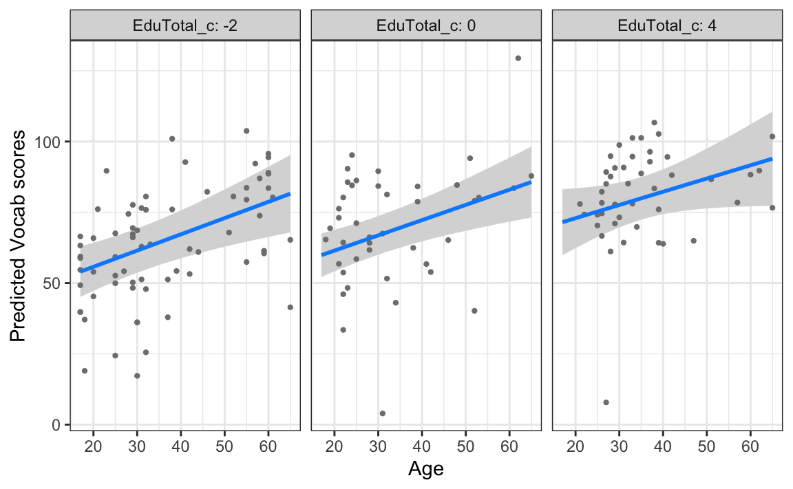
Vocab scores as predicted by model6 for English speakers of various ages who were in formal education for a below-average, average, and above-average length of time (in blue) and partial model residuals (grey points)
Examining Figure 13.6, we can therefore conclude that the effect of age on Vocab scores is not moderated by the number of years that participants spent in formal education.
The visreg() function provides two ways to visualise interaction effects between two numeric variables: in Figure 13.6, below-average, average, and above-average number of years in formal education were visualised across three panels. Figure 13.7 shows the same predictions but, this time, the code includes the argument “overlay = TRUE”, which results in a single panel with three coloured regression lines superimposed. This can make it easier to check whether the lines are parallel. From Figure 13.7, it is easier to see that the three lines are pretty much parallel to each other. This suggests that the positive effect of Age on Vocab scores does not change as a function of the number of years that participants were in formal education.
visreg(model6,
       xvar = "Age_c",
       by = "EduTotal_c",
       overlay = TRUE,
       xtrans = function(x) x + median(Dabrowska.data$Age),
       gg = TRUE) +
  labs(x = "Age",
       y = "Predicted Vocab scores") +
  theme_bw()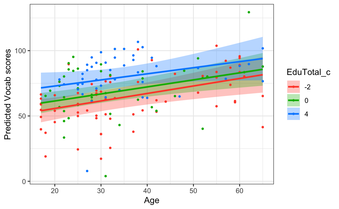
Vocab scores as predicted by model4_c for English speakers of various ages who were in formal education for a below-average (red line), average (green line), and above-average (blue line) period of time and partial model residuals (coloured points).
In order to interpret the output of a model featuring a significant interaction between two numeric predictors, we will now fit a simpler model predicting the Vocab scores of the L1 participants only (L1.data) using only two predictor variables: years in formal education (EduTotal) and Author Recognition Test (ART) scores.
The Author Recognition Test (Acheson, Wells & MacDonald 2008) is a measure of print exposure to literature, which is known to be a strong predictor of vocabulary knowledge (see Your turn! section in Section 13.4.1 above). This is confirmed in the L1 dataset as ART and Vocab scores are strongly correlated:
cor(L1.data$ART, L1.data$Vocab)[1] 0.6032758At the same time, we also know that there is a positive, though less strong, correlation between the number of years that L1 participants were in formal education and their Vocab test results:
cor(L1.data$EduTotal, L1.data$Vocab)[1] 0.4268695In the following, we explore the possibility that this positive association between Author Recognition Test (ART) scores and Vocab scores may be moderated by the number of years spent in formal education (EduTotal). If this interaction effect were negative, this would mean that, if two individuals both have the same high ART score, but one spent longer in formal education, then the effect of those extra years of education would not be as strong as they would be for someone with a lower ART score. To test this hypothesis, we formulate the following null hypothesis:
- H0: The number of years spent in formal education does not moderate the association of L1 English speakers’
ARTscores with theirVocabscores.
We now fit a model to find out if we have enough evidence to reject this null hypothesis:
# First, we center the numeric variables in the L1 dataset:
L1.data <- L1.data |>
   mutate(EduTotal_c = EduTotal - median(EduTotal),
          Blocks_c = Blocks - median(Blocks),
          Age_c = Age - median(Age))

# Second, we fit the model with both variables and their two-way interaction as predictors:
L1.model <- lm(Vocab ~ ART + EduTotal_c + ART:EduTotal_c,
              data = L1.data)

# Finally, we inspect the model:
summary(L1.model)
Call:
lm(formula = Vocab ~ ART + EduTotal_c + ART:EduTotal_c, data = L1.data)

Residuals:
    Min      1Q  Median      3Q     Max
-54.807  -6.113   0.065  10.927  26.379

Coefficients:
               Estimate Std. Error t value Pr(>|t|)
(Intercept)     51.9162     2.7622  18.795  < 2e-16 ***
ART              1.3088     0.1955   6.696 2.09e-09 ***
EduTotal_c       5.2626     1.3272   3.965 0.000151 ***
ART:EduTotal_c  -0.1803     0.0530  -3.402 0.001017 **
---
Signif. codes:  0 '***' 0.001 '**' 0.01 '*' 0.05 '.' 0.1 ' ' 1

Residual standard error: 15.18 on 86 degrees of freedom
Multiple R-squared:  0.4625,    Adjusted R-squared:  0.4437
F-statistic: 24.67 on 3 and 86 DF,  p-value: 1.311e-11
The model summary confirms that both predictors individually (i.e. as main effects) make statistically significant, positive contributions to the prediction of Vocab scores. Crucially, the summary also indicates that the interaction effect (ART:EduTotal_c) is statistically significant at α = 0.05 (p = 0.001017). The negative coefficient estimate of -0.1803 means that, for each additional year of formal education, our model predicts that the effect of a participant’s ART score on Vocab decreases by 0.1803 points. In simpler terms, the positive effect of reading literature, as measured by the Author Recognition Test (Acheson, Wells & MacDonald 2008), decreases slightly for every year spent in formal education.
Remember that, whenever we report an interaction, we can no longer interpret the estimated coefficients of the individual predictors in isolation. That is because we must also consider the interaction effect. To understand what this means in practice, let’s compare two speakers from the L1 dataset:
L1.data |>
  slice(2, 18) |>
  select(Occupation, OccupGroup, ART, EduTotal, Vocab)
Occupation OccupGroup ART EduTotal Vocab
1 Student/Support Worker PS 31 13 95.55556
2 Housewife I 31 17 84.44444Participant No. 2 is a student and support worker with an ART score of 31 points, who has (so far) spent 13 years in formal education.
Participant No. 18 is a housewife who also scored 31 points on the ART, but who was in formal education for a total of 17 years.
In general, we can calculate the Vocab scores that our L1.model predicts by combining the model’s coefficient estimates like this:
Intercept +
ARTcoefficient*ARTscore +
EduTotalcoefficient*(EduTotalin years - medianEduTotal) +
ART:EduTotalcoefficient*ARTscore*(EduTotalin years - medianEduTotal)
Based on the coefficient estimates of the model summary, we can therefore calculate the predicted Vocab score of the student / support worker as follows:
51.9162 +
1.3088 * 31 +
5.2626 * (13 - median(L1.data$EduTotal)) +
-0.1803 * 31 * (13 - median(L1.data$EduTotal))- 1
- Intercept coefficient
- 2
- Main effect of 31 points on the ART test
- 3
- Main effect of 13 years in formal education
- 4
- Interaction effect between 31 points on the ART and having spent 13 years in formal education
[1] 92.489And similarly for the housewife with the same ART score:
51.9162 +
1.3088 * 31 +
5.2626 * (17 - median(L1.data$EduTotal)) +
-0.1803 * 31 * (17 - median(L1.data$EduTotal))- 1
- Intercept coefficient
- 2
- Main effect of 31 points on ART test
- 3
- Main effect of 17 years in formal education
- 4
- Interaction effect between scoring 31 points on the ART and having spent 17 years in formal education
[1] 91.1822We can check that we did the maths correctly by checking the model’s prediction for these two individuals. Remember that minor differences after the decimal point are due to us using rounded coefficient estimates.
predict(L1.model)[2] 2
92.49038 predict(L1.model)[18] 18
91.18172 Notice how these two predicted scores are very similar, even though the housewife spent longer in formal education than the student / support worker. This is because, for L1 speakers, greater print exposure and more education generally lead to a larger vocabulary (as indicated by the positive main-effect coefficient estimates in L1.model), but the increase in vocabulary for each additional year of education is predicted to be smaller for individuals with higher ART scores.
Figure 13.8 visualises the predictions of L1.model. How can we interpret these three regression lines?
Show code to generate plot.
visreg(L1.model,
       xvar = "EduTotal_c",
       by = "ART",
       xtrans = function(x) x + median(L1.data$EduTotal),
       gg = TRUE) +
  labs(x = "Years in formal education",
       y = "Predicted Vocab scores") +
  theme_bw()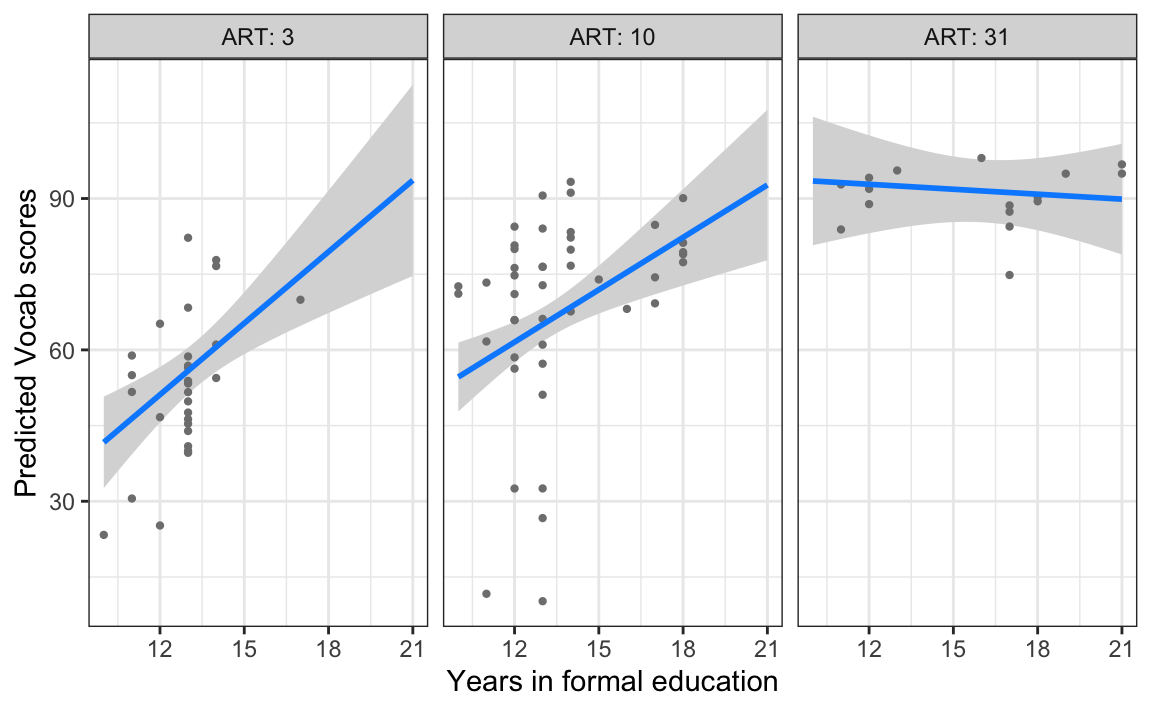
Vocab scores as predicted by L1.model (in blue) and partial model residuals (grey points) as a function of the number of years speakers were in formal education and for three ART test scores
For low and mid-level ART scores, the model predicts a positive correlation between the number of years a participant has spent in formal education and their predicted Vocab scores. However, this is not the case for participants who scored high on the ART test (third panel). The three regression lines representing the model’s predicted scores are clearly not parallel, and it would not be possible to draw three parallel lines that each stay within their respective 95% confidence bands. This confirms that, in this L1 model, the interaction between ART scores and years in formal education is statistically significant at α = 0.05. The main effects of these two predictors cannot be meaningfully interpreted without considering this interaction.
13.7 Model selection
Typically, the more predictors we enter in a model, the better the model fits the data. However, having predictors that contribute very little to the model and/or whose contributions are not statistically significant risks lowering the accuracy of the model’s predictions on new data. In this case, we say that the model overfits. A model that overfits the sample data risks not generalising to other data. If the aim of our statistical modelling is to infer from our sample to the general population (see Chapter 11), it can sometimes make sense to try to find an ‘optimal’ model that accounts for as much of the variance in the outcome variable as possible, relying only on association effects that we can be fairly confident could not have occurred due to chance only. This is where model selection comes into play.
Some people consider model selection to be a bit of an art. This chapter only aims to introduce the topic and does not cover — let alone compare or endorse — different model selection procedures. Ultimately, what really matters is that, if we intend to apply a model selection procedure, we decide on the method before analysing the data. The most credible way to settle on a model selection procedure prior to data analysis is to preregister an analysis plan on an online platform such as AsPredicted.org, Open Science Framework (OSF), and Zenodo (see Haroz 2022):
Preregistration [or pre-registration] is the practice of posting a time-stamped, read-only version of your study plan to a public repository before beginning data collection or analysis. This establishes a transparent record of your research intentions (Center for Open Science 2025).

Model selection bears the very real risk of (consciously or unconsciously) “fishing” for statistically significant results. Fishing is a highly Questionable Research Practice (QRP, see Section 11.7) that consists in trying out different methods until we arrive at findings that match our theory and/or hypotheses. For this reason, selection procedures in regression modelling have been heavily criticised over the years and there are very good arguments for not engaging in any model selection at all (Thompson 1995; Smith 2018; Harrell 2015: Section 4.3).
A fundamental problem with stepwise regression is that some real explanatory variables that have causal effects on the dependent variable may happen to not be statistically significant, while nuisance variables may be coincidentally significant. As a result, the model may fit the data well in-sample, but do poorly out-of-sample (Smith 2018: 1).
Nonetheless, in the following section, we will see how we might - if we decide to narrow down predictor variables using model selection - arrive at an optimal model of Vocab scores among L1 and L2 speakers of English using the adjusted R2 as our model selection decision criterion. Recall that R2 values correspond to the amount of variance in the outcome variable that a model can predict. The adjusted R2 is particularly useful because it is adjusted for the number of predictors entered in the model; models with more predictors are penalised.
When using adjusted R2 as the decision criterion, we seek to eliminate or add predictors depending on whether they lead to the largest improvement in adjusted R2 and we stop when adding or eliminating another predictor does not lead to further improvement in adjusted R2.
Adjusted R2 describes the strength of a model fit, and it is a useful tool for evaluating which predictors are adding value to the model, where adding value means they are (likely) improving the accuracy in predicting future outcomes. (Çetinkaya-Rundel & Hardin 2026: Section 8.4)
There are two common ways to add or remove predictors in a multiple regression model. These are called backward elimination and forward selection. They are often called stepwise selection because they add or remove one variable at a time.
Backward elimination starts with the full model – the model that includes all potential predictor variables. Predictors are eliminated one-at-a-time from the model until we cannot improve the model any further.
Forward selection is the reverse of the backward elimination technique. Instead of eliminating predictors one-at-a-time, we add predictors one-at-a-time until we cannot find any predictors that improve the model any further. (Çetinkaya-Rundel & Hardin 2026: Section 8.4)
We will use backward elimination as it allows us to start with a full model that includes all the predictors and any interactions that we believe are justified on the basis of theory and/or prior research. At this stage, it is absolutely crucial to think about which variables and which interactions are genuinely meaningful and which are not!
With the Dąbrowska (2019) data, several full models can be justified. In this section, we will attempt to model Vocab scores among L1 participants using four predictors (ART, Blocks_c, Age_c, EduTotal_c, and OccupGroup) and the following four interactions (ART:EduTotal_c, Blocks_c:EduTotal_c, ART:Age_c, and Blocks:Age_c). We can justify this choice of predictors based on our current understanding of language learning.
L1.model.full <- lm(Vocab ~ ART + Blocks_c + Age_c + EduTotal_c + OccupGroup + ART:EduTotal_c + Blocks_c:EduTotal_c + ART:Age_c + Blocks_c:Age_c,
           data = L1.data)

summary(L1.model.full)
Call:
lm(formula = Vocab ~ ART + Blocks_c + Age_c + EduTotal_c + OccupGroup +
    ART:EduTotal_c + Blocks_c:EduTotal_c + ART:Age_c + Blocks_c:Age_c,
    data = L1.data)

Residuals:
    Min      1Q  Median      3Q     Max
-42.927  -4.064  -0.374   8.295  28.282

Coefficients:
                      Estimate Std. Error t value Pr(>|t|)
(Intercept)         53.1677121  3.7269444  14.266  < 2e-16 ***
ART                  1.1304963  0.2330505   4.851 6.16e-06 ***
Blocks_c             1.4066157  0.3164938   4.444 2.88e-05 ***
Age_c                0.5955643  0.1895092   3.143  0.00237 **
EduTotal_c           4.4423564  1.3560678   3.276  0.00157 **
OccupGroupI          4.0757889  4.7833634   0.852  0.39678
OccupGroupM          0.1584647  4.3523775   0.036  0.97105
OccupGroupPS         0.4096426  4.3947432   0.093  0.92597
ART:EduTotal_c      -0.1523719  0.0513417  -2.968  0.00398 **
Blocks_c:EduTotal_c -0.1428729  0.1311735  -1.089  0.27942
ART:Age_c           -0.0125418  0.0096286  -1.303  0.19656
Blocks_c:Age_c      -0.0007549  0.0194954  -0.039  0.96921
---
Signif. codes:  0 '***' 0.001 '**' 0.01 '*' 0.05 '.' 0.1 ' ' 1

Residual standard error: 13.45 on 78 degrees of freedom
Multiple R-squared:  0.6172,    Adjusted R-squared:  0.5632
F-statistic: 11.43 on 11 and 78 DF,  p-value: 2.492e-12
Our full model has an adjusted R2 of 0.5632, which means that the combination of these variables and the four interactions account for about 56% of the variance in Vocab scores in the L1 data. However, many of the model coefficients in L1.model.full are not statistically significant, so we could try to remove them to see whether this leads to a lower adjusted R2 or not. Strictly speaking, a stepwise selection procedure would entail removing each interaction one-by-one. To save space here, we remove all three non-significant interaction terms in a single backward step:
L1.model.back1 <- lm(Vocab ~ ART + Blocks_c + Age_c + EduTotal_c + OccupGroup + ART:EduTotal_c,
           data = L1.data)

summary(L1.model.back1)
Call:
lm(formula = Vocab ~ ART + Blocks_c + Age_c + EduTotal_c + OccupGroup +
    ART:EduTotal_c, data = L1.data)

Residuals:
    Min      1Q  Median      3Q     Max
-42.282  -4.835   0.367   8.867  29.110

Coefficients:
               Estimate Std. Error t value Pr(>|t|)
(Intercept)    53.61458    3.60809  14.860  < 2e-16 ***
ART             0.97262    0.20158   4.825 6.48e-06 ***
Blocks_c        1.37827    0.31278   4.407 3.19e-05 ***
Age_c           0.42996    0.13122   3.276  0.00155 **
EduTotal_c      4.17372    1.30919   3.188  0.00204 **
OccupGroupI     4.00028    4.65106   0.860  0.39228
OccupGroupM     0.74751    4.29748   0.174  0.86235
OccupGroupPS   -0.22682    4.17410  -0.054  0.95680
ART:EduTotal_c -0.13709    0.04903  -2.796  0.00646 **
---
Signif. codes:  0 '***' 0.001 '**' 0.01 '*' 0.05 '.' 0.1 ' ' 1

Residual standard error: 13.38 on 81 degrees of freedom
Multiple R-squared:  0.6067,    Adjusted R-squared:  0.5679
F-statistic: 15.62 on 8 and 81 DF,  p-value: 1.153e-13
This procedure has actually led to a (very) small increase in our adjusted R2, which is now 0.5679, or 57%. Can we simplify our model even further and still account for as much variance in Vocab scores by dropping categorical predictor variable OccupGroup?
L1.model.back2 <-  lm(Vocab ~ ART + Blocks_c + Age_c + EduTotal_c + ART:EduTotal_c,
           data = L1.data)

summary(L1.model.back2)
Call:
lm(formula = Vocab ~ ART + Blocks_c + Age_c + EduTotal_c + ART:EduTotal_c,
    data = L1.data)

Residuals:
    Min      1Q  Median      3Q     Max
-43.379  -5.410   0.824   8.369  32.573

Coefficients:
               Estimate Std. Error t value Pr(>|t|)
(Intercept)     54.2022     2.4512  22.113  < 2e-16 ***
ART              0.9970     0.1922   5.187 1.46e-06 ***
Blocks_c         1.3251     0.3030   4.373 3.49e-05 ***
Age_c            0.4843     0.1092   4.434 2.78e-05 ***
EduTotal_c       4.3116     1.2812   3.365  0.00115 **
ART:EduTotal_c  -0.1472     0.0471  -3.125  0.00244 **
---
Signif. codes:  0 '***' 0.001 '**' 0.01 '*' 0.05 '.' 0.1 ' ' 1

Residual standard error: 13.21 on 84 degrees of freedom
Multiple R-squared:  0.6025,    Adjusted R-squared:  0.5788
F-statistic: 25.46 on 5 and 84 DF,  p-value: 1.521e-15
This new model has a slightly higher adjusted R2 (0.5788), so it looks like this was another sensible simplification of our model. All of the remaining coefficient estimates in L1.model.back2 make statistically significant contributions to the model. If we try to remove one, we can expect that the amount of variance that our model can account for will drop. For example, we can try to remove Age as a predictor from our model to see what happens:
L1.model.back3 <- lm(Vocab ~ ART + Blocks_c + EduTotal_c + ART:EduTotal_c,
           data = L1.data)

summary(L1.model.back3)
Call:
lm(formula = Vocab ~ ART + Blocks_c + EduTotal_c + ART:EduTotal_c,
    data = L1.data)

Residuals:
    Min      1Q  Median      3Q     Max
-48.816  -7.486  -0.458   9.970  26.546

Coefficients:
               Estimate Std. Error t value Pr(>|t|)
(Intercept)    52.08245    2.65487  19.618  < 2e-16 ***
ART             1.38099    0.18951   7.287  1.5e-10 ***
Blocks_c        0.90754    0.31806   2.853  0.00543 **
EduTotal_c      3.59093    1.40344   2.559  0.01228 *
ART:EduTotal_c -0.15028    0.05201  -2.890  0.00489 **
---
Signif. codes:  0 '***' 0.001 '**' 0.01 '*' 0.05 '.' 0.1 ' ' 1

Residual standard error: 14.59 on 85 degrees of freedom
Multiple R-squared:  0.5095,    Adjusted R-squared:  0.4864
F-statistic: 22.07 on 4 and 85 DF,  p-value: 1.615e-12
Indeed, L1.model.back3 accounts for 49% of the variance (adjusted R2 = 0.4864), which is considerably less than L1.model.back2. We will therefore report and interpret L1.model.back2.
NoteReporting a multiple regression model
There are many ways to report the numerical results of a statistical model. Researchers typically include a table reporting the model’s coefficient estimates (sometimes referred to as β, “beta”), together with a measure of variability around these estimates (e.g. standard error or confidence intervals), as well as their associated p-values. In addition, it is important to report the accuracy of the model. Different so-called goodness-of-fit measures are used for this; one of the most common being the adjusted coefficient of determination, R2. The output of the summary() function includes all of these statistics and is therefore suitable for a research report.
Alternatively, the {sjPlot} library (Lüdecke 2020) includes a handy function that produces nicely formatted tables to report all kinds of models, including multiple linear regression models. When you run the tab_model() function in RStudio, the table will be displayed in the Viewer pane. By default, it includes the model’s coefficient estimates and 95% confidence intervals around these estimates, as well as p-values formatted in bold if they are below 0.05.
install.packages("sjPlot")
library(sjPlot)

tab_model(L1.model.back2)| Vocab | |||
|---|---|---|---|
| Predictors | Estimates | CI | p |
| (Intercept) | 54.20 | 49.33 – 59.08 | <0.001 |
| ART | 1.00 | 0.61 – 1.38 | <0.001 |
| Blocks c | 1.33 | 0.72 – 1.93 | <0.001 |
| Age c | 0.48 | 0.27 – 0.70 | <0.001 |
| EduTotal c | 4.31 | 1.76 – 6.86 | 0.001 |
| ART × EduTotal c | -0.15 | -0.24 – -0.05 | 0.002 |
| Observations | 90 | ||
| R2 / R2 adjusted | 0.603 / 0.579 | ||
Check the documentation of the tab_model() function and the sjPlot website to learn about its many useful formatting options:
?tab_modelIt is also recommended to visualise the model’s predictions and its (partial) residuals. Again, there are many ways to achieve this in R, but we will stick to using the {visreg} library. Run the following command and follow the instructions displayed in the Console to view all the plots in RStudio. You may need to resize your Plot pane or use the Zoom button to properly view the plots.
visreg(L1.model.back2)Running the visreg() function on this multiple regression model outputs several warning messages in the Console. These messages are important and should not be ignored:
Note that you are attempting to plot a 'main effect' in a model that contains an interaction. This is potentially misleading; you may wish to consider using the 'by' argument.The message warns us that we should not attempt to interpret ART and EduTotal_c as main effects because our model includes an interaction that involves these two variables. Indeed, the fourth plot (see Figure 13.9) suggests that the more years an L1 speaker spends in formal education, the greater their Vocab score; however, because our model includes an interaction effect, the authors of the {visreg} package are warning us that the strength or even the direction of this effect could change depending on individuals’ ART score.
visreg(fit = L1.model.back2,
       xvar = "EduTotal_c",
       xtrans = function(x) x + median(L1.data$EduTotal),
       gg = TRUE) +
  labs(x = "Years in formal education",
       y = "Predicted Vocab scores") +
  theme_bw()
Conditions used in construction of plot
ART: 10.5
Blocks_c: 0
Age_c: 0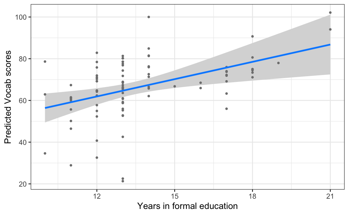
As suggested by the warning message, we can (and should!) visualise interactions like this one using the “by” argument.
visreg(fit = L1.model.back2,
       xvar = "EduTotal_c",
       xtrans = function(x) x + median(L1.data$EduTotal),
       by = "ART",
       gg = TRUE) +
  labs(x = "Years in formal education",
       y = "Predicted Vocab scores") +
theme_bw() 
Figure 13.10 shows the predicted effect of the number of years in formal education on Vocab scores for participants who scored 3, 10, and 31 points on the ART. The regression line shows a positive relation between Vocab scores and years in formal education for below-average and average ART scores, but the regression line is almost flat for above-average ART scores. This indicates that, for individuals who score very high on the ART, years in education is no longer a useful predictor of their Vocab scores.
Finally, we should also report the outcome of our model assumption checks. This is covered in the following section.

13.8 Checking model assumptions
As we saw in Section 12.4, it is crucial that we check that our models meet the assumptions of linear regression models before we interpret them because, if they don’t, our models may be unreliable. In some cases, modelling issues may already be visible from the model summary. Warning signs include very large model residuals, coefficient estimates reported as NA, and warning messages stating that the model is “singular” or that it has “failed to converge”.
These problems can occur for a number of reasons, but most often because the model is too complex given the data available: the sample size may be too small or the data too sparse for certain combinations of predictors (e.g. if you try to enter gender and native language as predictors in a model, but for some languages only female native speakers are represented in the dataset). There are often ways around these issues, but they are beyond the scope of this introductory textbook (see recommended readings below and next-step resources).
The model assumptions for multiple linear regression models are the same as for simple linear regression models (see Section 12.4):
- Independence of the data points (see Section 11.6.2 and Section 12.4.1)
- Linear relationships between the predictors (see Section 11.6.4 and Section 12.4.2)
- Homogeneity of the model residuals (see Section 11.6.5 and Section 12.4.3)
- Normality of the model residuals (see Section 11.6.3)
- No overly influential outliers (see Section 11.6.4)
There is only one additional assumption that is specific to models that include multiple predictors:
- No multicollinearity
In the following, we use the check_model() function from the {performance} package (Lüdecke, Ben-Shachar, et al. 2021) to check these assumptions graphically. The check_model() function also requires the installation of the {qqplotr} (Almeida, Loy & Hofmann 2018) and {see} (Lüdecke, Patil, et al. 2021) packages to work.

install.packages(c("performance", "qqplotr", "see"))
library(performance)
Running the function on the saved model object should generate a large figure comprising six plots2 (see Figure 13.11). In the following, we will learn to interpret them one-by-one.
check_model(L1.model.back2)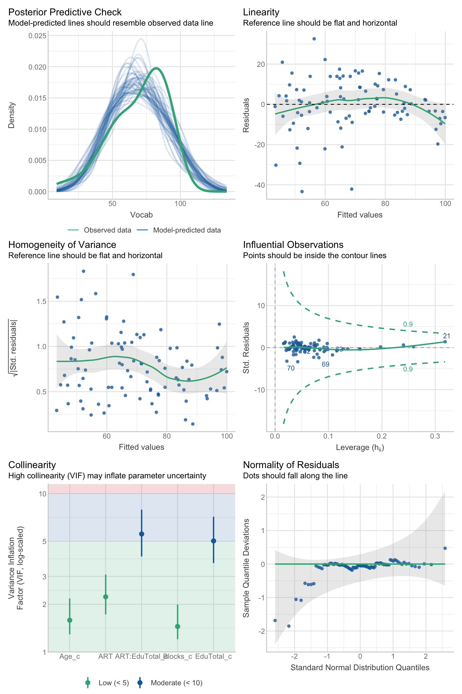
check_model() function for assessing key assumptions of linear regression models
By default, check_model() outputs a single figure that allows us To check the most important model assumptions. This large figure is useful for reporting purposes, but it is rather unwieldy for interpretation. Changing the “panel” argument of the check_model() function to FALSE returns a list of {ggplot} objects that we can save to our local environment as diagnostic.plots:
diagnostic.plots <- plot(check_model(L1.model.back2, panel = FALSE))Then we can use the double square bracket operator to display a single diagnostic plot from this saved list:
diagnostic.plots[[1]]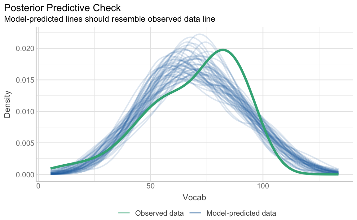
This first plot (Figure 13.12) is another way to compare the model’s predicted values (represented here as blue distributions) with the real-life (i.e observed) outcome variable (represented here in green). We can see that the center of the distribution of observed Vocab scores is slightly shifted to the right compared to most distributions of model-predicted data. That said, the simulated distributions are close to the real distribution and largely follow a similar shape. If they didn’t, this would suggest that a linear regression model may not be suitable for our data.
The second plot (Figure 13.13) is designed To check the assumption of linearity. If the predictors are linearly related, the green reference line should be flat and horizontal. Our reference line is slightly curved, but it remains possible to draw a horizontal line through the grey band, hence we can conclude that the assumption of linearity is not severely violated.
diagnostic.plots[[2]]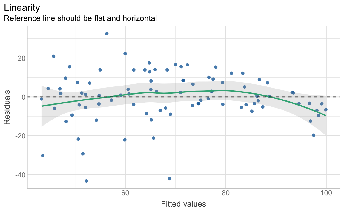
Note that Figure 13.13 is actually the same kind of plot as Figure 12.11 that we generated to check the assumption of equal (or constant) variance, i.e. homoscedasticity. Fitted values is another term for predicted values. Thus, in Figure 13.13, the x-axis represents the Vocab scores predicted by the model. When the assumption of homoscedasticity is met, the model residuals are randomly distributed above and below 0, i.e. they do not notably increase or decrease as predicted values increase.
The {performance} package proposes a different kind of diagnostic plot to check the assumption of homoscedasticity (see Figure 13.14) with the square-root of the absolute standardised residuals on the y-axis. A roughly flat and horizontal green reference line indicates homoscedasticity. Again, although the reference line in Figure 13.14 is by no means perfectly flat, a flat line can be drawn within the grey band, suggesting that the assumption is met.
diagnostic.plots[[3]]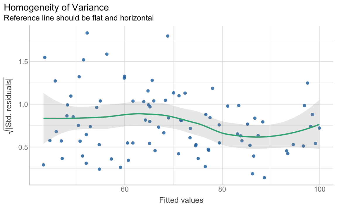
The fourth diagnostic plot (Figure 13.15) helps to detect outliers in the data that may have a particularly strong influence on our model. It is based on Cook’s distance (see Levshina 2015: Section 7.2.4; Sonderegger 2023: Section 5.7.3). Any points that fall outside the dashed green lines fall outside Cook’s distance and are considered influential observations.
diagnostic.plots[[4]]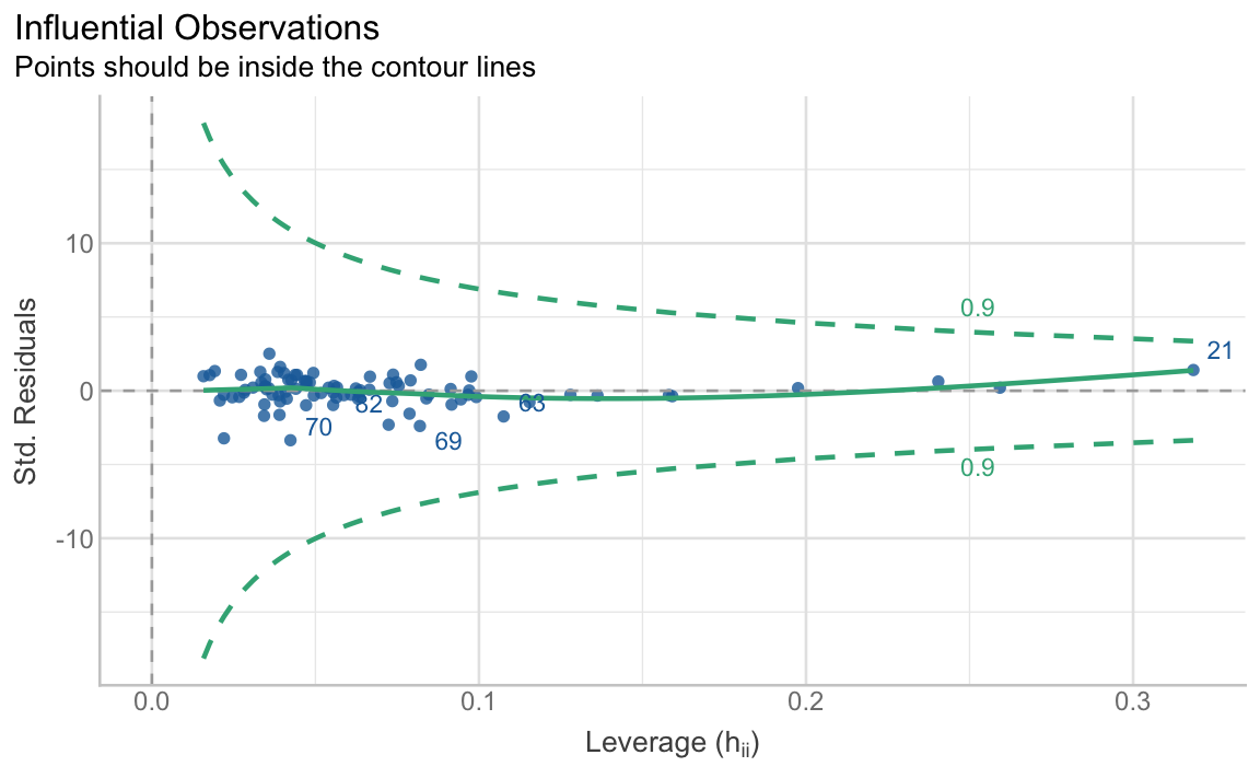
In Figure 13.15, no data point falls outside of Cook’s distance so we are not concerned about influential observations violating the assumptions of our model. Still, it is interesting to briefly explore the most influential observations, which are labelled by their index number in the dataset. In Figure 13.15, one of these is participant number 21:
L1.data |>
  slice(21) |>
  select(Age, Gender, Occupation, Blocks, EduTotal, ART, Vocab)
Age Gender Occupation Blocks EduTotal ART Vocab
1 41 F Senior Lecturer 9 21 43 93.33333As you can see, this female senior lecturer is rather unusual: she performed below average in the non-verbal IQ test (Blocks), yet achieved the second-highest Vocab score. She also performed far above average on the author recognition test (ART) and reported the longest period in formal education among the L1 participants (EduTotal).
In some cases, it may be justified to remove overly influential outliers; however, this should typically only be done when we are fairly certain that the outliers were caused by a technical error, such as a measuring instrument not functioning properly, or a human error, such as a participant misunderstanding the direction of a response scale. All other outliers may be theoretically interesting: if our aim is to generalise our model to the full population, we must be prepared to include some unusual observations that also belong to that population. In the case of L1 English speakers, this includes people who spent more than 20 years in formal education and are seemingly much more into languages than the kind of abstract puzzles typically found in non-verbal IQ tests!
The fifth diagnostic plot output by the check_model() function (Figure 13.16) serves to check the assumption of a no multicollinearity. Multicollinearity, or high collinearity, refers to a strong linear dependence between predictors such that they do not contribute unique or independent information to the model. Multicollinearity should not be confused with a strong correlation between two individual predictors as measured using the cor.test() function (see Section 11.5). What matters here is the association between one or more predictor variables, conditional on the other variables in the model. This is considerably more complex to calculate, but luckily, there are several functions that allow us to do just that in R.
The {performance} package relies on the Variance Inflation Factor (VIF) to quantify collinearity. Typically, VIF scores above 10 are considered to indicate a problematic degree of collinearity between some predictors. Figure 13.16 indicates that our model does not suffer from multicollinearity.
diagnostic.plots[[5]]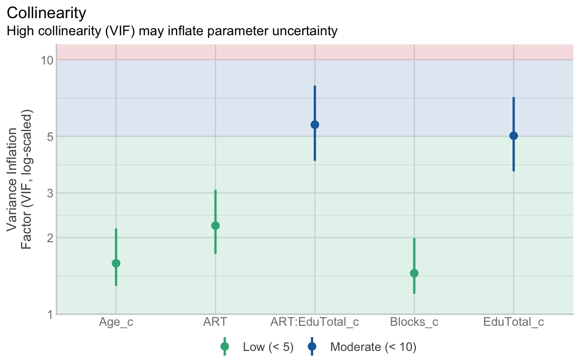
Finally, the sixth plot output by the check_model() function serves to check the assumption of the normality of the residuals. In Section 12.4.4, we achieved this by visualising the distribution of residuals as a density plot (see Figure 12.12). The diagnostic plot presented in Figure 13.17, by contrast, is a so-called Q-Q plot (quantile-quantile plot). These plots are designed to compare the shapes of distributions. If the residuals follow a perfect normal distribution, the points should all fall along the straight reference line (in green).
diagnostic.plots[[6]]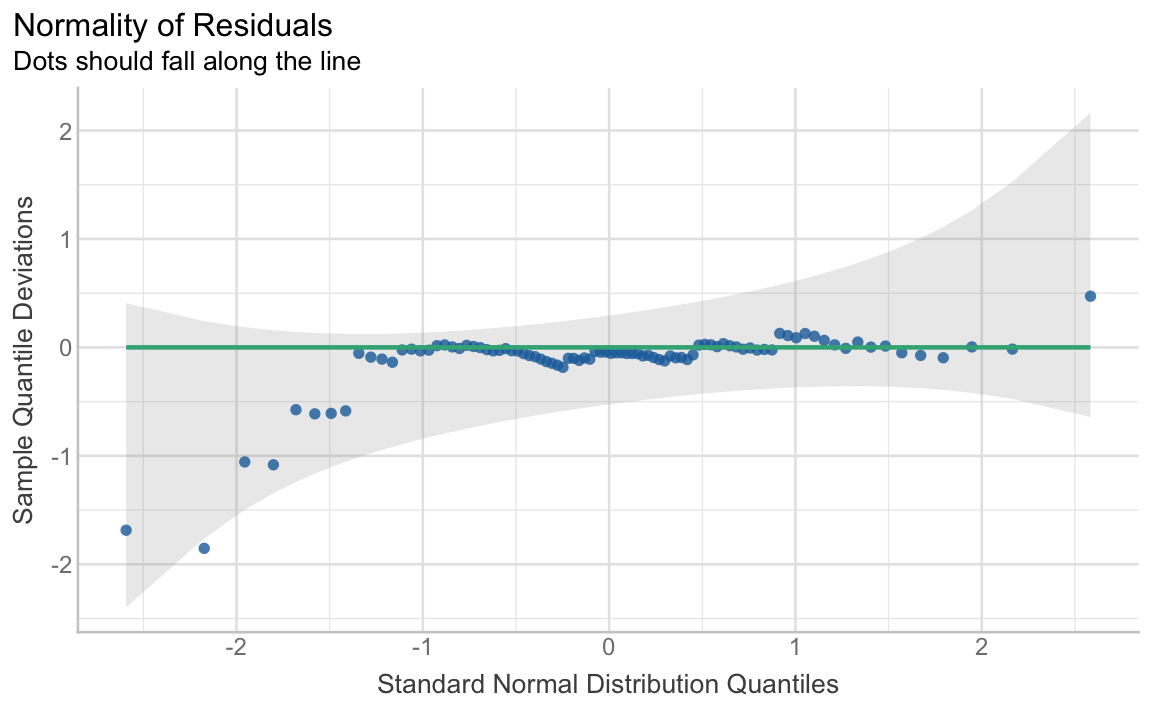
In Figure 13.17, we see that most residuals follow a normal distribution, except some observations at the tails of the distribution. This is fairly typical and, if the other model assumptions are not violated, minor deviations from normality like this are unlikely to be a problem, especially with larger sample sizes.
Note
The check_model() vignette provides more detailed information on these diagnostic plots, how to interpret them, and what to do if the assumptions are not met: https://easystats.github.io/performance/articles/check_model.html.
TipYour turn!
So far in this chapter, we have fitted a model of L1 speakers’ Vocab scores. We have found that participants’ print exposure (as measured by the ART), non-verbal intelligence (as measured by the Blocks test), their age, the number of years they were in formal education, and the interaction between ART scores and years in education all contribute to being able to predict how well they performed on the Vocab test. The model that we selected as the optimal model (L1.model.back2) was able to predict 58% of the variance in Vocab scores among L1 speakers.
In this task, your aim is to find out which predictors and interactions among predictors can be used to predict Vocab scores among L2 speakers and to what degree of accuracy. In addition to the predictors that we entered in our full L1 model, you can enter three additional predictors in your model that are relevant to L2 speakers only:
- Age at which they started living in an English-speaking country (
Arrival) - Total number of years they have been living in an English-speaking country (
LoR) - Number of hours they spend reading in English in a typical week (
ReadEng)
Run the following code to median-center some of these numeric variables in L2.data:
L2.data <- L2.data |>
  mutate(Blocks_c = Blocks - median(Blocks),
         Age_c = Age - median(Age),
         EduTotal_c = EduTotal - median(EduTotal),
         Arrival_c = Arrival - median(Arrival),
         LoR_c = LoR - median(LoR))
Then, fit the following multiple linear regression model on the L2 dataset and examine the model summary:
L2.model <- lm(formula = Vocab ~ ART + Blocks_c + Age_c + EduTotal_c + Arrival_c + LoR_c + ReadEng + ART:EduTotal_c + ART:ReadEng + EduTotal_c:ReadEng + Arrival_c:Age_c + LoR_c:Arrival_c,
             data = L2.data)

summary(L2.model)
Q13.10 How many interaction terms contribute to the predictions made by L2.model?
🐭 Click on the mouse for a hint.
Q13.11 Use the check_model() function to visually check whether L2.model meets the most important assumptions of multiple linear regression models. Which assumption(s) are obviously violated?
🐭 Click on the mouse for a hint.
Show sample code to answer Q13.11.
diagnostic.plots.L2 <- plot(check_model(L2.model, panel = FALSE))

diagnostic.plots.L2[[1]] # No issues here.

diagnostic.plots.L2[[2]] # Also no issues here.

diagnostic.plots.L2[[3]] # Nothing major to worry about: the reference line is not perfectly flat, but it's not far off.

diagnostic.plots.L2[[4]] # No observation points appear to have an overly large influence on the model

diagnostic.plots.L2[[5]] # Here we have three coefficients with VIF scores > 10. This is problematic!

diagnostic.plots.L2[[6]] # The residuals are not normally distributed, but the largest deviation is at lowest end of the distribution which is not terribly unusual.
We can display the exact VIF values of a model using the vif() function from the {car} package (Fox & Weisberg 2018):
install.packages("car")
library(car)

vif(L2.model)
ART Blocks_c Age_c EduTotal_c
5.987790 1.216035 25.347847 5.490682
Arrival_c LoR_c ReadEng ART:EduTotal_c
23.746278 11.102277 3.661388 2.237536
ART:ReadEng EduTotal_c:ReadEng Age_c:Arrival_c Arrival_c:LoR_c
8.550867 4.412402 3.349661 1.398937 From this list of VIF values, we can see that three predictors display high collinearity: Age_c, Arrival_c, and LoR_c. This makes sense because, for most L2 participants recruited in the UK, if we know how old they were when they arrived in the UK (Arrival), and their length of residence in the country in years (LoR), then we can probably almost predict their age (Age) to a high degree of accuracy. We can easily check this hypothesis in a random sample of six participants from our L2.data:
L2.data |>
  select(Arrival, LoR, Age) |>
  slice_sample(n = 6)
Arrival LoR Age
1 26 3 29
2 32 6 38
3 22 5 28
4 17 3 20
5 23 4 27
6 16 14 30As you can see, in most cases, participants’ age is equal to their age when they first arrived in the country plus the number of years they’ve been living there since. This is why Age and the combination of the predictors Arrival and LoR are almost perfectly correlated:
cor(L2.data$Age, (L2.data$Arrival + L2.data$LoR))[1] 0.9768833To remedy this, we must remove one of these three predictors from our model. Fit a new model that does not include participants’ age when they first arrived in the UK (Arrival). Save this new model as L2.model.b. Check that it now meets all the model assumptions and then examine its summary.
Q13.12 Adjusted for the number of predictors entered into L2.model.b, what percentage of the variance in Vocab scores in the L2 dataset does this model accurately predict?
Show sample code to answer Q13.12.
L2.model.b <- lm(formula = Vocab ~ ART + Blocks_c + Age_c + EduTotal_c + LoR_c + ReadEng + ART:EduTotal_c + ART:ReadEng + EduTotal_c:ReadEng,
             data = L2.data)

check_model(L2.model.b) # Now all looking much better than earlier!

summary(L2.model.b) # Adjusted R-squared:  0.2027
Q13.13 Which main-effect predictor(s) make a statistically significant contribution to L2.model.b at α = 0.05?
Q13.14 Does the model’s coefficient estimate for ReadEng make intuitive sense?
Q13.15 Which interaction effect(s) make a statistically significant contribution to L2.model.b at α = 0.05?
Q13.16 Use the {visreg} library to visualise the model’s predicted Vocab scores (on the y-axis) as a function of all possible ReadEng values (on the x-axis) and subdivide the figure into three panels corresponding to low, mid-level, and high ART scores. Which arguments do you have to use inside the visreg() function to achieve this?
🐭 Click on the mouse for a hint.
Show sample code to answer Q13.16.
visreg(fit = L2.model.b,
       xvar = "ReadEng",
       by = "ART")
13.9 Tapping into the potential of statistical modelling
This chapter aimed to provide first insights into the potential of statistical modelling with multiple predictors. It has demonstrated the importance of considering interactions between predictors and of visualising both the observed sample data, as well as simulated values based on the predictions of a statistical model.
You may have noted that p-values were not at the heart of this chapter. Instead, we focused on model accuracy (as measured by the adjusted R2), coefficient estimates and their relative importance (as measured by the lmg metric), predicted values, and (partial) model residuals. This is because there is an unfortunate tendency among some students and researchers to be misled into thinking that, if a result turns out to be statistically significant, it must be true. As statistician Andrew Gelman puts it, some confuse statistics for “a form of modern alchemy, transforming the uncertainty and variation of the laboratory and field measurements into clean scientific conclusions that can be taken as truth” (Gelman 2018: 43).
I hope that working through Chapter 11 to 13 has shown you that a big part of learning to work with quantitative data in the language sciences is really about “embracing variation and accepting uncertainty” (Gelman 2019). If we intend to report inferential statistics based on sample data, it is important that we decide on significance level thresholds, model selection criteria, and other such parameters before conducting our data analysis (on the benefits of preregistrating protocols and methods in the language sciences, see e.g. Mertzen, Lago & Vasishth 2021; Roettger 2021). If we want to test hypotheses, these must be well-defined hypotheses and we must strive to quantify (and ideally also visualise!) uncertainty. Ultimately, it is worth remembering that “in almost all practical data analysis situations – we can only draw uncertain conclusions from data, regardless of whether we manage to obtain statistical significance or not” (Vasishth & Gelman 2021: 1311). Crucially, we must be extremely careful when extrapolating our results beyond the range of our observed data.
As explained in Chapter 11, statistical inference based on NHST and p-values comes from a statistical framework called frequentism, which happens to (currently) be the most widely used framework in the language sciences. Taking a frequentist approach means that the statistical properties of the hypothesis tests that we conduct are considered under hypothetical replications of our study with new sample data. This is because, in the frequentist framework, we estimate the long-run probability of observing certain effects, were we to repeat the study many times. This is one of the reasons why replication (see Section 14.2) is key to advancing our knowledge of linguistics and language teaching and learning. Whenever we have small sample sizes, small effect sizes (i.e. small coefficient estimates in statistical models), large measurement error, and/or lots of variability among the target population – as is often the case in the language sciences – we simply cannot get reliable results from a single sample.
Does this mean that we should give up with quantitative data analysis and statistics all together? No, of course not. On the contrary, this uncertainty makes research in the language sciences all the more interesting and worth pursuing! It also means that there is much more to be learnt in terms of methods. In this chapter, you have learnt about frequentist fixed-effects linear regression models. These models are incredibly useful and can be used in many contexts, but they make a number of important assumptions that do not always hold:
Perhaps the most obvious, yet one that we have not discussed so far, is that the outcome variable of a linear regression model must be quantitative, like the
Vocabvariable inDabrowska.data, which ranges from -13.33 to 95.56 (see Section 7.2). Other types of statistical models can be used to model other types of outcome variables, including:Binomial (or binary) logistic regression models allow us to predict binary outcomes (e.g. whether or not a verb is negated) (to find out more, see e.g. Levshina 2015: Chapter 12; Sonderegger 2023: Chapter 6; Winter 2019: Chapter 12).
Multinomial logistic regression models can be used to model categorical outcome variables with more than two levels (e.g. which modal verb is used in certain constructions) (to find out more, see e.g. Levshina 2015: Chapter 13).
Poisson regression models are used to model count variables, i.e. discrete numeric variables such as the frequency of fillers (such as uh and oh) in certain contexts (to find out more, see e.g. Winter 2019: Chapter 13).
The observations (i.e. the data points) used to fit a fixed-effect model must be independent of each other. In the language sciences, such a situation is actually quite rare (see Section 12.4.1). To model interdependencies between observations, we can fit mixed-effects models (also called multilevel or hierarchical models) (to learn more, see e.g. Vasishth et al. 2022; Sonderegger 2023: Chapters 8-10; Winter 2019: Chapters 14-15).
Linear regression models assume linear relationships between the predictors. There are different ways to circumvent this problem. In some cases, predictors can be transformed to meet this assumption (see Winter 2019: Chapter 5). In others, it may be wiser to model non-linear associations with other kinds of models such as Generalised Additive Mixed Models Wieling (2018).
Finally, we need not stick to the frequentist school of statistics. In fact, quantitative linguists are increasingly turning to Bayesian statistics and finding that Bayesian models help them work with the particularities of linguistic data (to learn more about Bayesian statistics, see e.g. Levshina 2022; Nicenboim, Schad & Vasishth 2025).
NoteRecommended further reading 📚
In this textbook, we have only just scratched the surface of statistical modelling. We can do much, much more with these kinds of models, and there are lots of additional things to take into account. The good news is that there are lots of excellent resources to help you continue your statistical modelling journey. Here are some good places to get started (in alphabetical order):
- Gries, Stefan Thomas. 2021. Statistics for linguistics with R: A practical introduction (De Gruyter Mouton Textbook). 3rd revised edition. De Gruyter Mouton.
- Levshina, Natalia. 2015. How to do linguistics with R: Data exploration and statistical analysis. John Benjamins.
- Nicenboim, Bruno, Daniel Schad & Shravan Vasishth. 2026. Introduction to Bayesian Data Analysis for cognitive science (Chapman & Hall/CRC Statistics in the Social and Behavioral Sciences Series). CRC Press. Open Access version: https://bruno.nicenboim.me/bayescogsci/.
- Sonderegger, Morgan. 2023. Regression modeling for linguistic data. Cambridge, Massachusetts: The MIT Press. Open Access version: https://osf.io/pnumg/.
- Winter, Bodo. 2020. Statistics for Linguists: An Introduction Using R. Routledge.
Although they go further than the present textbook, you will also find that these resources begin by explaining many of the things already covered in this chapter and previous chapters, and that’s actually a good thing. There’s no harm in revising these complex topics from a different perspective, with different examples, R packages, and coding styles.
Check your progress 🌟
Congratulations: you have successfully completed the most difficult chapter of this textbook! 💪 You have answered 0 out of 16 questions correctly.
Are you confident that you can…?
Loading the {relaimpo} package returns several warnings informing us, on the one hand, about packages that {relaimpo} requires to work and which are therefore also automatically loaded (these are called dependencies) and, on the other, about objects being masked by different packages, e.g.:
The following object is masked from ‘package:dplyr’:

select
It is worth paying attention to the latter set of warnings because it means that some function names, e.g.
select(), are now shared by more than one package in ourRenvironment. This can cause code that previously worked fine to suddenly return errors. For example, after loading the {relaimpo} package, you may find that theselect()function no longer works as expected becauseRattempts to use theselect()function from the {MASS} package rather than from the tidyverse {dplyr} package. To avoid this happening, we can manually assign the correct package to the function name like this:select <- dplyr::selectThis ensures that any future mentions of the
select()function are, by default, interpreted as the function defined in the {dplyr} package.↩︎If your version of RStudio does not display the six-panelled figure but instead only a white canvas, this is probably because your Plots pane is too small. In this case, you will need to make it as large as possible and then try running the function again. If that doesn’t work either, don’t worry as we will save and examine individual plots from now on.↩︎