library(here)
library(tidyverse)19 LeaRning Direction Effects in Retrieval Practice on EFL Vocabulary Learning
NoteAbout the authors of this chapter
Hannah Boxleitner is a first-year master’s student in linguistics at the University of Cologne. After completing her first bachelor’s degree in social work in Regensburg, and mostly working in the field of social services, she studied linguistics and German studies at the University of Cologne, where she focused on metaphor studies and corpus linguistics. She has now additionally taken an interest to computational linguistics within the specialization of her master’s.
Beyhan Aliy is a first-year master’s student in linguistics at the University of Cologne, where she specializes in psycho- and neurolinguistics. She also completed her bachelor’s degree in linguistics and English studies at the University of Cologne. She is currently working as a student assistant at the Department of Linguistics.
The authors made equal contributions to the chapter. An earlier version of this chapter was submitted as a term paper for Elen Le Foll’s M.A. seminar “Introduction to Data Analysis in R for linguists and language education scholars” (University of Cologne, summer 2025). Elen supervised the project, provided feedback, and contributed to the present revised version of this chapter.
Chapter overview
This chapter aims to reproduce the analyses published in:
Terai, Masato, Junko Yamashita, and Kelly E. Pasich. 2021. EFFECTS OF LEARNING DIRECTION IN RETRIEVAL PRACTICE ON EFL VOCABULARY LEARNING. Studies in Second Language Acquisition 43(5): 1116–1137. https://doi.org/10.1017/S0272263121000346.
Based on the original data from Terai, Yamashita & Pasich (2021), we show how R can be used in Second Language Acquisition (SLA) research. This chapter will walk you through how to:
- Retrieve the authors’ original data and import it in
R - Calculate descriptive statistics concerning target items, test types, and alpha coefficients for tests
- Reproduce Tables 3, 4 and 5 from Terai, Yamashita & Pasich (2021)
- Fit a generalized linear mixed-effects model to investigate the effectiveness of learning direction
- Compare models with and without interactions
- Fit a generalized linear mixed-effects model to explore the influence of L2 proficiency on the two types of learning
- Interpret and compare the results with those published in Terai, Yamashita & Pasich (2021)
- Visualize the results with different kinds of plots to facilitate interpretation
By the end of this chapter, you will have experience of fitting and interpreting mixed-effects logistics regression models in R on experimental data.
19.1 Introducing the study
In this chapter, we attempt to reproduce the results of an SLA study by Terai, Yamashita & Pasich (2021). The study focuses on learning directions in pair-associated vocabulary learning: L2 to L1, where L2 words are used as stimuli and responses are given in L1 vs. L1 to L2, where it is the other way around. As opposed to studying practices where both a target and the answer are simultaneously presented, pair-associated learning involves retrieval. Retrieval is defined as the process of accessing stored information and plays a crucial role in retaining a learned word in memory (Terai, Yamashita & Pasich 2021: 1116-1117). Previous findings regarding the efficacy of the two types of learning directions had been inconsistent. The study that we will reproduce focuses on the relationship between L2 proficiency and the effectiveness of the two learning directions in paired-associate learning in L2 vocabulary acquisition. It aims to answer two research questions:
- Which learning direction is more effective for vocabulary acquisition, L1 to L2 learning or L2 to L1 learning?
- How does L2 proficiency influence the effects of L2 to L1 and L1 to L2 learning?
To answer these questions, Terai, Yamashita & Pasich (2021) designed an experiment in which Japanese EFL (English as a Foreign Language) learners studied word pairs and then completed retrieval practice tasks in different conditions. After learning, students were tested on their ability to produce the target vocabulary items in both Japanese (their L1) and English (their L2). Terai, Yamashita & Pasich (2021) formulated two hypotheses:
- There is no significant difference between the two learning directions.
- The effect of the learning direction depends on the learner’s L2 proficiency (Terai, Yamashita & Pasich 2021: 1121-1122).
19.2 Retrieving the original data
We will use the study’s original data for our reproduction, which the authors have made openly accessible on IRIS, an open-access database for language research data and materials.
Not only have the authors made their research data available, they have also shared their R code. Our reproduction will examine and run this R code to investigate and interpret the statistical analyses and results presented in the original publication.
The dataset (dataset1_ssla_20210313.csv) contains data for each participant and item, including the following key variables:
- Answer (whether the participant gave the correct answer (1 = correct, 0 = incorrect))
- Test (distinguishing the two test types: L1 Production and L2 Production)
- Condition (distinguishing the two learning directions: L2 -> L1 or L1 -> L2)
But more on that later.
19.3 Set-up and Data import
Before importing the dataset and starting on our project, we need to load all the packages that we will need. You may have to first install some of these packages using the install.packages() command in your console.
Next, we import the data. In contrast to Terai, Yamashita & Pasich (2021)’s code, we used the {here} package for importing the data. This package creates paths relative to the top-level directory and therefore makes it easier to reference files in a reproducible manner (see Section 6.5).
VocabularyA_L1production <- read.csv(file = here("B_CaseStudies", "Hannah-Beyhan", "data", "vocaA_L1pro_20210313.csv"))
VocabularyA_L2production <- read.csv(file = here("B_CaseStudies", "Hannah-Beyhan", "data", "vocaA_L2pro_20210313.csv"))
VocabularyB_L1production <- read.csv(file = here("B_CaseStudies", "Hannah-Beyhan", "data", "vocaB_L1pro_20210313.csv"))
VocabularyB_L2production <- read.csv(file = here("B_CaseStudies", "Hannah-Beyhan", "data", "vocaB_L2pro_20210313.csv"))

# Loading the dataset
dat <- read.csv(file = here("B_CaseStudies", "Hannah-Beyhan", "data", "dataset1_ssla_20210313.csv"), header=T)
As already mentioned, the dataset contains different information on items and participants. The other four files contain the vocabulary scores for each item, for both L1 and L2 production tests and both Vocabulary A and Vocabulary B items. Every cell contains either 1 (correct) or 0 (incorrect).
19.4 Descriptive statistics
Before we dive into the descriptive statistics conducted in Terai, Yamashita & Pasich (2021), we need to explain that one part of it will not be reproduced. While descriptive statistics about the participants (age, years of learning, etc.) are mentioned in the original paper (Terai, Yamashita & Pasich 2021: 1122-1123), we were not able to find the data to reproduce these findings. That said, it is common for participant data not to be shared to protect their identities. Therefore, in this section, we will focus on reproducing the descriptive statistics of the target items (40 English words used in the study), test types and reliability testing. We’ll start with the target items, which are found in Table 3 in the paper (Terai, Yamashita & Pasich 2021: 1123).
Most of the numbers reproduced here are statistics already introduced in the textbook: mean, median, maximum and minimum, as well as the standard deviation (SD) (see Chapter 8). In addition, Terai, Yamashita & Pasich (2021) report skewness and kurtosis. Skewness and kurtosis are both measures of the shape and distribution of a variable. Skewness measures the asymmetry of a distribution. Simply put, skewness describes the proportion of a distribution which differs from a completely symmetrical shape (Parajuli 2023):
- Skew = 0 -> perfectly symmetrical.
- Negative Skew -> longer “tail” on the left.
- Positive Skew -> longer “tail” on the right.
Kurtosis is a measure of peaks of a distribution. Basically, it is a description of how the peaks compare to a normal distribution (Parajuli 2023):
- Kurtosis = 0 -> similar to a normal distribution.
- Positive kurtosis -> sharper peak (more concentrated in the center).
- Negative kurtosis -> flatter peak. (Parajuli 2023)
19.4.1 Reproduction of Table 3
In this section, our aim is to reproduce Table 3 from Terai, Yamashita & Pasich (2021): 1123, which displays the descriptive statistics of the target items of the study. Unfortunately, the code for all the tables shown in Terai, Yamashita & Pasich (2021) was not included in the shared R code. But as we have the data in the form of a .csv file, this is not a problem! We have the organized data ready for us to analyze. Thus, we will learn how to reproduce the data of Table 3 step-by-step.
In the following chunk, we load some necessary libraries and use the trimws() function, which removes space from the beginning and end of the text. This helps to prevent issues like “berth” vs. “berth” being treated as two different word forms.
# Load libraries (packages need to first be installed, if they aren't already)

library(moments) #for skewness and kurtosis
library(knitr) #for nice tables
library(kableExtra) #for nicer tables

dat$ItemID <- trimws(dat$ItemID)
In the paper by Terai, Yamashita & Pasich (2021) we can see that the variables for the English (L2-related variables) words they used are: Frequency, Syllables, and Letters. For Japanese (L1-related variables): Frequency, Letters, and Mora (syllables) as well as Familiarity (Fami A). Fami (A) refers to familiarity ratings taken from the large database by Amano & Kondo (2000) as the authors explain (Terai, Yamashita & Pasich 2021: 1123). These ratings showed how familiar each Japanese word is to the general population. The second familiarity ratings (Fami (B)), represents the participants’ own familiarity ratings collected for this study. We were not able to reproduce Fami (B) as the data was not made public.
Show the R code to generate the table below.
var_info <- data.frame(
  Column = c("ItemID", "L2Frequency", "Syllables", "Alphabet", "L1Frequency", "WordLength", "mora", "Familiarity"),
  Description = c(
    "English target word (40 items)",
    "Frequency of the word in English (COCA: Corpus of Contemporary American English)",
    "Number of syllables in the English word",
    "Number of letters in the English word ('Letters' in the L2 table)",
    "Frequency of the word in Japanese (Amano & Kondo, 1999)",
    "Number of letters in the Japanese orthographic form",
    "Number of mora (Japanese syllable-like units)",
    "Participants Familiarity ratings from current study (Fami (B))"
  )
)

kable(var_info) %>%
kable_styling(full_width = FALSE, position = "center")| Column | Description |
|---|---|
| ItemID | English target word (40 items) |
| L2Frequency | Frequency of the word in English (COCA: Corpus of Contemporary American English) |
| Syllables | Number of syllables in the English word |
| Alphabet | Number of letters in the English word ('Letters' in the L2 table) |
| L1Frequency | Frequency of the word in Japanese (Amano & Kondo, 1999) |
| WordLength | Number of letters in the Japanese orthographic form |
| mora | Number of mora (Japanese syllable-like units) |
| Familiarity | Participants Familiarity ratings from current study (Fami (B)) |
Basically, what we are doing next is reshaping our data from participant-focused to item-focused. The raw dataset has multiple rows per word because each participant contributed several responses and thus has their own row per word. For example, the word “weasel” appears many times, once for each participant. But to compute descriptive statistics of the items, we only want one row per word.
To solve this issue we use the functions group_by() and summarise() to turn all those rows into just a single one per word. With group_by(ItemID), we group all rows together that contain the same word. Combining the summarise() and first() functions then creates our new dataset by keeping only the first mention of each word’s frequency, number of syllables, etc. Only for the familiarity ratings do we calculate the mean() across all participants as word familiarity differs across the participants. The last argument .groups = "drop" removes the grouping structure so that the resulting dataset is no longer grouped by ItemID.
items <- dat |>
  group_by(ItemID) |>
  summarise(
    L2Frequency = first(L2Frequency),
    Syllables = first(Syllables),
    Alphabet = first(Alphabet),
    L1Frequency = first(L1Frequency),
    WordLength = first(WordLength),
    mora = first(mora),
    familiarity = mean(familiarity, na.rm = TRUE),
    .groups = "drop"
  )
We want to do a quick check before we continue: Did we correctly import all 40 target words from the study (as described in Terai, Yamashita & Pasich 2021: 1123) into our items dataframe?
nrow(items)[1] 40With this command we can also see what kind of words the authors were examining:
head(items, 5)# A tibble: 5 × 8
ItemID L2Frequency Syllables Alphabet L1Frequency WordLength mora familiarity
<chr> <int> <int> <int> <int> <int> <int> <dbl>
1 alcove 932 2 6 178 4 4 5.53
2 azalea 450 3 6 230 3 3 5.81
3 badger 818 2 6 6 4 4 3.94
4 berth 1851 1 5 245 4 4 5.53
5 billow 231 2 6 362 4 4 5.16In order to avoid repeating code (and because we are lazy), we created our own function that computes all the descriptive statistics (mean, SD, median, min, max, skew, kurtosis) we need for each variable. We write our own function to do so (which you can think of as a “small machine”) that we will name quick_stats() and that will do the calculations for us. quick_stats <- funcion(x) creates this function with the input ‘x’ which represents whichever variable we want to analyze. Inside of our function, we use data.frame() to organize our statistics before we begin the calculations. Each function within our function takes our input variable ‘x’ and computes the statistics. The functions skewness() and kurtosis() come from the {moments} package that we loaded earlier.
quick_stats <- function(x) {
  data.frame(
    Mean = mean(x, na.rm = TRUE),
    SD = sd(x, na.rm = TRUE),
    Median = median(x, na.rm = TRUE),
    Minimum = min(x, na.rm = TRUE),
    Maximum = max(x, na.rm = TRUE),
    Skew = moments::skewness(x, na.rm = TRUE),
    Kurtosis = moments::kurtosis(x, na.rm = TRUE)
    )
}
Now that we have most of what we need for the tables, we can start to build them up! We need to create two subtables.
The code below does this with two important functions: rbind() which stacks the rows we want to create on top of each other to build the final table which we will print in the next step. And cbind() which creates columns that stick together side by side. For example cbind(Variable = "Frequency", desc(items$L2Frequency) creates a column with the name “Variable” with the value “Frequency” next to the summary of the output of quick_stats(). With our helper function desc() we then insert the statistics from our data, in this case it is the “L2Frequency”. Basically, we are creating here three rows stacked on top of each other for tab_L2, and four rows for tab_L1. As you see we only have to run our helper function quick_stats() seven times!
tab_L2 <- rbind(
  cbind(Variable = "Frequency", quick_stats(items$L2Frequency)),
  cbind(Variable = "Syllables", quick_stats(items$Syllables)),
  cbind(Variable = "Letters", quick_stats(items$Alphabet))
)

tab_L1 <- rbind(
  cbind(Variable = "Frequency", quick_stats(items$L1Frequency)),
  cbind(Variable = "Letters", quick_stats(items$WordLength)),
  cbind(Variable = "Mora (syllables)", quick_stats(items$mora)),
  cbind(Variable = "Fami (A)", quick_stats(items$familiarity))
)
Perfect, the next and easiest part of building up our two subtables is captioning them and then finally printing them. Here we need the kable() and the kable_classic() function. We use these functions to make the tables look easy to read. The kable() function is quite nice because it helps to make the R code output look a little more professional. The function comes from the {knitr} package. kable(tab_L2, ...) takes our tab_2 data frame and converts it into a formatted table which we then caption with the argument caption = "...". With the argument align = "lrrrrrr" we control the way the text is aligned in each column. the ‘l’ means left-aligned, while every added “r” means the remaining columns should be right-aligned. With the argument digits = 2 we display all numeric values to a maximum of two decimal places.
The kable_classics() function comes from the {kableExtra} package we loaded earlier. It is also another function to tidy up our table style. The command full_width = FALSE makes sure that the table does not stretch too wide. When you run this code, you will see a nice table with clear structure and formatting which will make it easier to read and interpret, it also looks ready to be published.
kable(tab_L2,
      align = "lrrrrrrr",
      digits = 2) |>
kable_classic(full_width = FALSE)| Variable | Mean | SD | Median | Minimum | Maximum | Skew | Kurtosis |
|---|---|---|---|---|---|---|---|
| Frequency | 1025.33 | 851.93 | 813.5 | 51 | 3930 | 1.51 | 5.21 |
| Syllables | 2.00 | 0.91 | 2.0 | 1 | 5 | 0.84 | 4.06 |
| Letters | 6.22 | 1.75 | 6.0 | 3 | 12 | 0.97 | 4.52 |
kable(tab_L1,
      align = "lrrrrrrr",
      digits = 2) |>
kable_classic(full_width = FALSE)| Variable | Mean | SD | Median | Minimum | Maximum | Skew | Kurtosis |
|---|---|---|---|---|---|---|---|
| Frequency | 596.90 | 885.49 | 275.00 | 6.00 | 5109.00 | 3.59 | 18.10 |
| Letters | 3.67 | 1.07 | 4.00 | 1.00 | 6.00 | 0.17 | 3.48 |
| Mora (syllables) | 3.52 | 0.96 | 4.00 | 1.00 | 6.00 | 0.19 | 4.29 |
| Fami (A) | 5.22 | 0.64 | 5.36 | 3.72 | 6.38 | -0.63 | 2.83 |
Our reproduced tables Table 19.2 and Table 19.3 now closely match Table 3 (Terai, Yamashita & Pasich 2021: 1123)! The L2 frequency has a mean of about 1025 with a quite large SD (~852), which shows us that some English words were quite frequent while others were much rarer. The skewness is positive (~1.51), although slightly different than the one reported in the paper (~1.57). The difference is only small and still shows that the distribution has a “long tail” of very high-frequency words. English words are, on average, 2 syllables, and range from 1 to 5 syllables with only a slight positive skewness which means that most words are short and only a few are longer. Again we note a small difference in our skewness metric compared to the one reported in the original study. On average, words are 6.2 letters long, again with a positive skewness. For the L1 variables, the frequency distribution also shows a strong positive skew, which means that few Japanese words are very common, but many are quite rare. Fami (A) averages about 5.2 on a 7-point scale, with a pretty low SD, suggesting that the words were mostly familiar, meaning participants generally recognized these Japanese words easily.
Our skewness values match the original paper fairly closely, with only small differences. However, our kurtosis values differ quite a lot from the published results. This may seem like a huge issue at first, but is actually quite normal. Kurtosis calculations can vary between packages, for example the {moments} package we used calculates excess kurtosis, while the authors of the original paper might have used a different method. We tried several methods to reproduce the kurtosis values from the original publication, but failed to produce the values reported in the original study. We calculated both the excess kurtosis and the pearson kurtosis (see code chunk below), but no numbers match the ones in the paper.
# Instead of mora any other variable of Table 3 can be added to calculate kurtosis
excess_kurt <- kurtosis(dat$mora, na.rm = TRUE)
pearson_kurt <- excess_kurt + 3
round(c(excess = excess_kurt, pearson = pearson_kurt), 3)
excess pearson
4.285 7.285 There are several possibilities why this is the case. There might be an outlier that may have been removed, or maybe the authors used another method. The issue with the differences in our numbers and the ones by Terai, Yamashita & Pasich (2021) is that the differences are so big the graphs are going to look quite different, especially for the Fami (A) variable. In the original paper, the kurtosis shows -0.02 which would be a slightly flatter graph, while our kurtosis number 4.29 would be sharper. This is why, in an extension, we have added some graphs to show the importance of skewness and kurtosis and what exactly these numbers show.
NoteExtension: Visualizations of Table 3
Table 3 from the original study displays a summary of many descriptive statistics (mean, SD, range, skewness, kurtosis) for the 40 target words, but these numbers are much easier to understand when they are visualized. Below we want to turn some key variables of Table 3 into quick histograms to visually connect the ideas of skewness and kurtosis to the actual items used in this study.
# The {tidyverse} library needs to be loaded if you have not done it before.

items <- dat |>
  group_by(ItemID) |>
  summarise(
    L2Frequency  = first(L2Frequency),
    Syllables    = first(Syllables),
    Letters_L2   = first(Alphabet),
    L1Frequency  = first(L1Frequency),
    Letters_L1   = first(WordLength),
    Mora         = first(mora),
    Familiarity  = mean(familiarity, na.rm = TRUE),
    .groups = "drop"
  )
We will start with a graph of L2 Frequencies. To do this we use the ggplot() command. The first line of code here ggplot(data = items, aes(x = L2Frequency)) tells ggplot to basically use the “items” dataset and put the L2 frequencies of each word onto the x-axis. geom_density(...) creates the actual density plot. To fully understand where the numbers in the table come from, we add reference lines: geom_vline(xintercept = mean(...)) for the mean value, and geom_vline(xintercept = median(...), linetype = "dashed"...) for a dashed line at the median.
Do not be too confused by the numbers on the y-axis. The values can be read as a kind of probability, a higher peak means more words are around that frequency, while a lower peak means fewer words around that frequency.
ggplot(items, aes(x = L2Frequency)) +
  geom_density(fill = "lightblue") +
  geom_vline(xintercept = mean(items$L2Frequency), linewidth = 0.7) +
  geom_vline(xintercept = median(items$L2Frequency), linetype = "dashed", linewidth = 0.7) +
  scale_y_continuous(labels = scales::comma) +
  scale_x_continuous(labels = scales::comma) +
  labs(x = "L2 frequency (COCA)",
       y = "Probability") +
theme_minimal()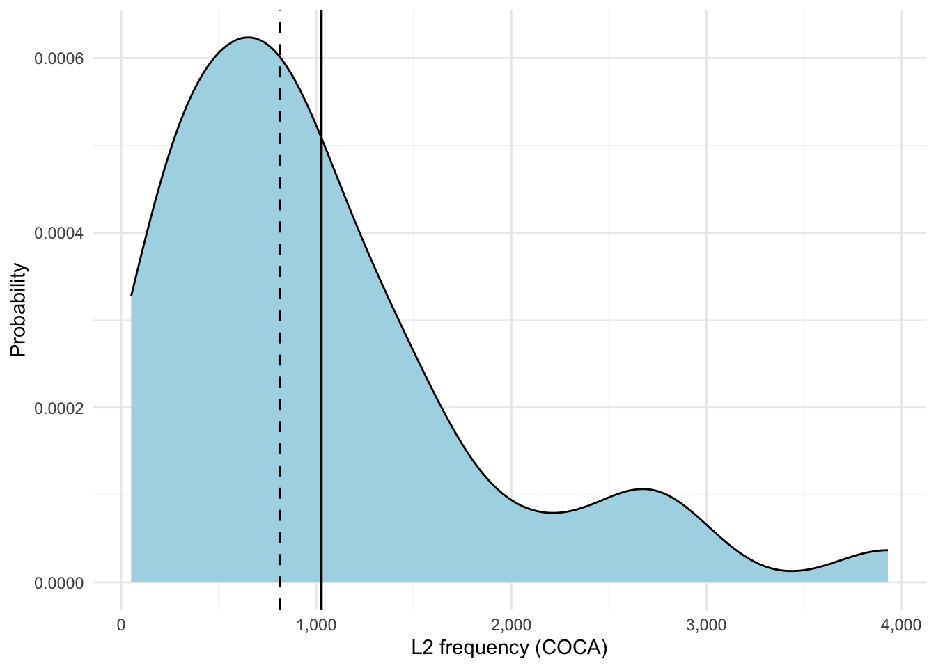
In Figure 19.1 we can clearly see a right-skewed distribution which we saw in the table with the positive skewness values (~1.51). As you may recall, a normally distributed graph would look like a symmetric bell curve. By contrast, here, we see that most words have lower or medium frequency with only a few really high-frequency words (see the long right tail). The mean sits to the right of the median which is another characteristic of positive skew. Our kurtosis value (~5.21) shows us the sharpness or peakedness of our curve which you can see quite nicely when you compare the graph for L2 frequency to the one for L1 frequency (see Figure 19.2).
ggplot(items, aes(x = L1Frequency)) +
  geom_density(fill = "lightblue") +
  geom_vline(xintercept = mean(items$L1Frequency), linewidth = 0.7) +
  geom_vline(xintercept = median(items$L1Frequency), linetype = "dashed", linewidth = 0.7) +
  scale_x_continuous(labels = scales::comma) +
  scale_y_continuous(labels = scales::comma) +
  labs(x = "L1 frequency",
       y = "Probability",
       caption = "Solid line = mean; dashed line = median") +
theme_minimal()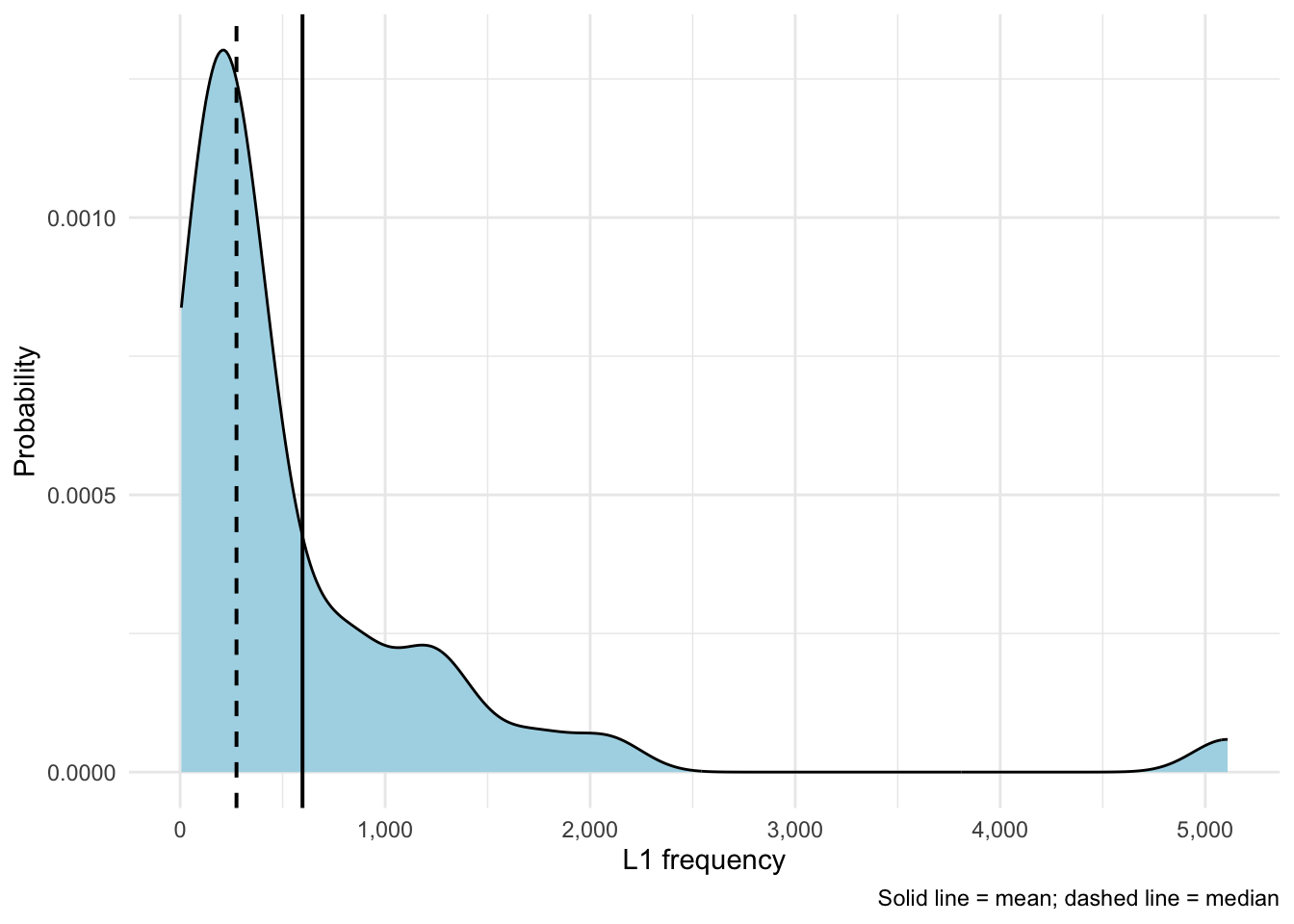
Figure 19.2 shows that a right-skew that is even stronger than for L2 word frequencies (skew ~3.59). This shows once again that most words are lower-frequency, there are only very few high-frequency words. Here, with a kurtosis value of ~18.10 we can see that with higher positive numbers the peak becomes sharper and sharper.
19.4.2 Descriptive statistics of the tests and reliability testing
In this section, we will attempt to reproduce the authors’ descriptive statistics regarding the two types of post-tests and calculate Cronbach’s α to estimate their reliability.
19.4.2.1 Reliability analysis
To conduct reliability analysis, the {psych} package needs to be installed and loaded.
library(psych)To calculate Cronbach’s α, Terai, Yamashita & Pasich (2021) applied the alpha() function to the vocabulary scores of both the L1 and L2 production sets. Below, we only show the code of the reliability analysis for Vocabulary A scores of the L1 production dataset, as an example:
alpha(VocabularyA_L1production[,-1], warnings=FALSE)Show code for reliability analysis for the rest of the dataset
# Vocabulary A (L2 production)

alpha(VocabularyA_L2production[,-1], warnings = FALSE)

# Vocabulary B (L1 production)

alpha(VocabularyB_L1production[,-1], warnings = FALSE)

# Vocabulary B (L2 production)

alpha(VocabularyB_L2production[,-1], warnings = FALSE)
These reliability analyses compute Cronbach’s α, a measure of internal consistency of tests. This measure indicates whether responses are consistent across items. Before interpreting these results, we will get to the descriptive statistics of the two types of post-tests.
19.4.2.2 Accuracy
To investigate accuracy, Terai, Yamashita & Pasich (2021) processed the collected results for each participant — their ID, how many items they answered, and how many they got right — and visualized them as boxplots. In the original code, the authors loaded the dataset for this section again and stored it under a different object name dat.acc. We skipped that step and simply used dat instead as it is already available as an R object in our local environment.
The following code chunk, which analyses data pertaining to L2 -> L1 direction of the L1 production set, processes the results for each participant — their ID, answered items, correct answers — and puts them into a clean table. Therefore, it gives us the core numbers necessary to describe and analyze learners’ vocabularly retrieval accuracy.
# L2 → L1 (L1 production test)

z <- unique(dat$ID)

Score <- c()
IDes <- c()
try <- c()

for (i in z){
  dat |>
    dplyr::filter(ID == i, Condition == "L2L1", Test == "L1 Production") |>
    dplyr::select(Answer) -> acc_recT
  a <- as.vector(unlist(acc_recT))
  b <- sum(a)
  c <- length(a)
  Score <- c(Score, b)
  IDes <- c(IDes, i)
  try <- c(try, c)
}

accu_L2L1_L1Pro <- data.frame(IDes, try, Score)
names(accu_L2L1_L1Pro) <- c("ID", "Try", "Score")
accu_L2L1_L1Pro
We want to take the time to explain this code chunk in detail. The first line takes unique IDs from dat and saves it as z, z therefore being a vector of unique IDs. This part was slightly changed in comparison to Terai, Yamashita & Pasich (2021)’s code, which used three lines of code for this step. Further, a for loop is used to iterate over elements of this vector and assigning the IDs to the variable i. Inside this loop, for each i (a unique ID) the data is filtered for that participant under certain conditions, and then the Answer column is selected. The result is stored as the object acc_recT, which is further converted into a vector a. With b and c, the processed answers are computed and lastly, these results are appended into three vectors: Score, IDes, and try. These three vectors are combined into a final data frame accu_L2L1_L1Pro, where each vector becomes a column in a table, each row corresponding to one participant. These columns are renamed and the table is printed. If we want to properly see the table outside of the console, we can use the View() function:
View(accu_L2L1_L1Pro)For L1 -> L2 of the L1 production set, we follow the same steps.
Show code for L1 -> L2 (L1 production test)
# L1 → L2 (L1 production test)

z <- unique(dat$ID)

Score <- c()
IDes <- c()
try <- c()
for (i in z){
  dat |>
    dplyr::filter(ID == i, Condition =="L1L2", Test == "L1 Production") |>
    dplyr::select(Answer)-> acc_recT
  a <- as.vector(unlist(acc_recT))
  b <- sum(a)
  c <- length(a)
  Score <- c(Score, b)
  IDes <- c(IDes, i)
  try <- c(try, c)
}

accu_L1L2_L1Pro <- data.frame(IDes, try, Score)
names(accu_L1L2_L1Pro) <- c("ID", "Try", "Score")
accu_L1L2_L1Pro
While accuracy did not play a very big role in the published paper, the authors did a bit more with it in their code. Aside from using the describe() function on the final data frames, which returns a rich set of descriptive statistics, they visualized the results as boxplots. Since we found them to be quite nice for understanding the descriptive statistics of the tests, we decided to include these in this chapter, too.
Show use of describe() function on Score column to provide descriptive statistics for L1 production
# L2 → L1 learning
describe(accu_L2L1_L1Pro$Score)

# L1 → L2 learning
describe(accu_L1L2_L1Pro$Score)
To visualize descriptive statistics for the L1 production set, the authors generated boxplots comparing the two learning directions. For this to work, the {beeswarm} package has to be installed and loaded. The authors assigned a data frame L1pro that contains the scores from both learning directions in the L1 production test. After changing the names of the columns to how they shall appear on the x-axis, the authors created side-by-side boxplots for the two learning conditions. Finally, they added the beeswarm() function specifying add = T, which lets individual scores appear as jittered dots so that they don’t overlap.
# Plot (L1 production)

library(beeswarm)

L1pro <- data.frame(accu_L2L1_L1Pro$Score, accu_L1L2_L1Pro$Score)
names(L1pro) <- c("L2 → L1 learning", "L1 → L2 learning")
boxplot(L1pro, col = "grey91", outline = T)
beeswarm(L1pro, add = T)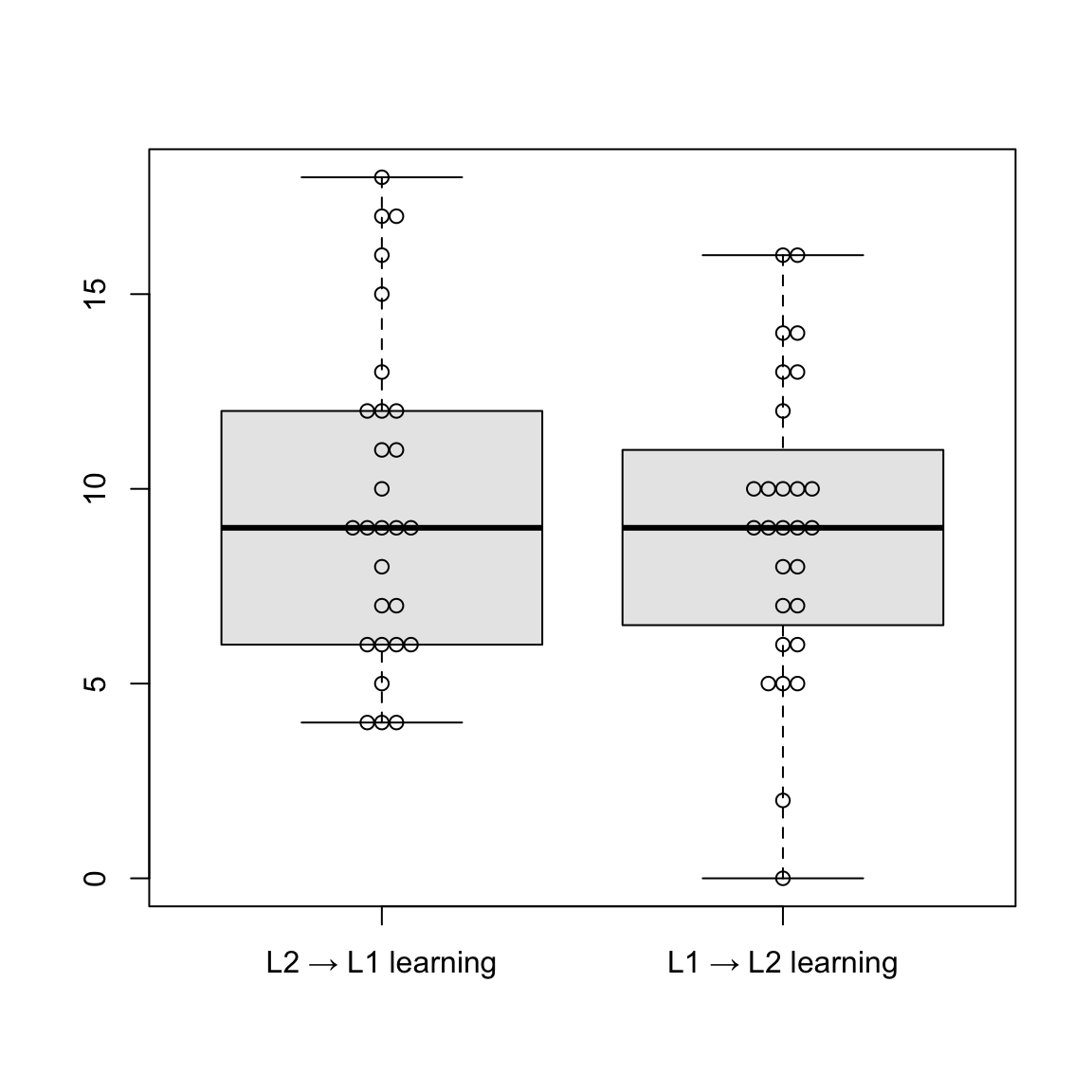
Boxplots are a way to visualize both the central tendency (median) of a variable and the spread around this central tendency (IQR) (see Section 8.3.2). The median is represented by the thick line inside the box, while the box represents interquartile range, meaning the range of the middle 50% of the data. The whiskers outside the box extend to the highest and smallest values, and the jittered dots represent individual data points. As we can see here, the median is similar in both learning directions. L2 → L1 displays slightly greater variability and a higher concentration of upper outliers. Overall, performance appears comparable between the two groups.
The same steps were applied to the L2 production set, using the L2 scores.
Show code for L2 → L1 (L2 production test)
# L2 → L1 (L2 production test)

z <- unique(dat$ID)

Score <- c()
IDes <- c()
try <- c()
for (i in z){
  dat |>
    dplyr::filter(ID == i, Condition == "L2L1", Test == "L2 Production") |>
    dplyr::select(Answer) -> acc_proT
  a <- as.vector(unlist(acc_proT))
  b <- sum(a)
  c <- length(a)
  Score <- c(Score, b)
  IDes <- c(IDes, i)
  try <- c(try, c)
}

accu_L2L1_L2Pro <- data.frame(IDes, try, Score)
names(accu_L2L1_L2Pro) <- c("ID", "Try", "Score")
accu_L2L1_L2Pro
Show code for L1 → L2 (L2 production test)
# L1 → L2 (L2 production test)

z <- unique(dat$ID)

Score <- c()
IDes <- c()
try <- c()
for (i in z){
  dat |>
    dplyr::filter(ID == i, Condition == "L1L2", Test == "L2 Production") |>
    dplyr::select(Answer)-> acc_proT
  a <- as.vector(unlist(acc_proT))
  b <- sum(a)
  c <- length(a)
  Score <- c(Score, b)
  IDes <- c(IDes, i)
  try <- c(try, c)
}

accu_L1L2_L2Pro <- data.frame(IDes,try, Score)
names(accu_L1L2_L2Pro) <- c("ID", "Try", "Score")
accu_L1L2_L2Pro
Show use of describe() function on Score column to provide descriptive statistics for L2 production
# L2 -> L1 learning

describe(accu_L2L1_L2Pro$Score)

# L1 -> L2 learning

describe(accu_L1L2_L2Pro$Score)
As with L1, Terai, Yamashita & Pasich (2021) created similar boxplots comparing the two learning directions in L2 production using the beeswarm package.
Show R code to generate boxplots
# Plot (L2 production)

L2pro <- data.frame(accu_L2L1_L2Pro$Score, accu_L1L2_L2Pro$Score)
names(L2pro) <- c("L2 → L1 learning", "L1 → L2 learning")
boxplot(L2pro, col = "grey91", outline = T)
beeswarm(L2pro, add = T)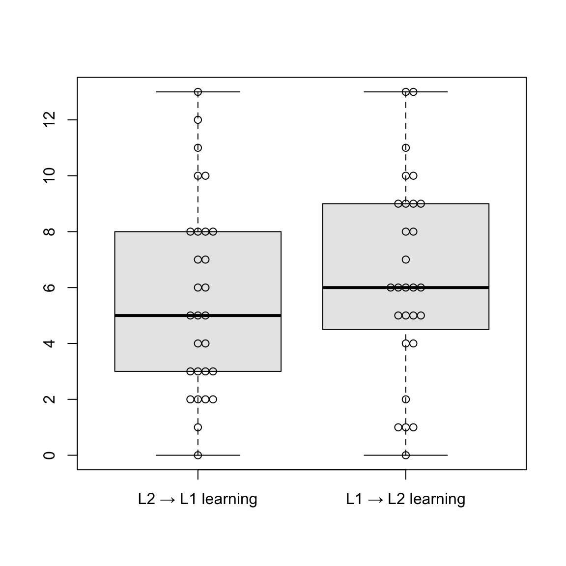
Median scores in the L2 production test are similar for both learning directions (L2 → L1 and L1 → L2), suggesting comparable performance in both groups. L1 → L2 learning shows a slightly higher median. In the L2 → L1 group, values below the median are more spread out, indicating more variety. Comparing the L1 and L2 production tests, L1 production scores appear to be generally higher and more consistent across both learning directions.
19.4.2.3 Reproducing Table 4 and 5
After conducting reliability testing and descriptive statistics for the tests, we want to display the results in tables like Tables 4 and 5 from the original publication (Terai, Yamashita & Pasich 2021: 1126). As with the target items, there was no code accessible for creating these tables. But with the available data, we can find a way to reproduce them anyway!
First, we want to create a table that summarizes results of descriptive statistics of tests, similar to Table 4 (Terai, Yamashita & Pasich 2021: 1126). The {knitr} and {kableExtra} packages have to be loaded to proceed. As a first step, we assign a variable that contains the scores for both datasets (L1 and L2 production) and use the describe() function to get all the important measures.
descriptive_stats_tests <- data.frame(L1pro, L2pro) |>
  describe()
To reproduce the original table, the first two columns (vars and n) are removed. Also, the rows are renamed to be more readable.
descriptive_stats_tests_trimmed <- descriptive_stats_tests |>
  select(-n, -vars, -trimmed, -mad, -range, -se)

rownames(descriptive_stats_tests_trimmed) <- c("L2 → L1 (L1pro)", "L1 → L2 (L1pro)", "L2 → L1 (L2pro)", "L1 → L2 (L2pro)")
Now we want to display the results in a clean, formatted table using the kable() function.
kable(descriptive_stats_tests_trimmed,
      digits = 2) |>
  pack_rows(index = c("L1 production test" = 2, "L2 production test" = 2)) |>
kable_styling(full_width = FALSE, bootstrap_options = c("striped", "hover"))| mean | sd | median | min | max | skew | kurtosis | |
|---|---|---|---|---|---|---|---|
| L1 production test | |||||||
| L2 → L1 (L1pro) | 9.71 | 4.16 | 9 | 4 | 18 | 0.44 | -0.92 |
| L1 → L2 (L1pro) | 9.00 | 3.85 | 9 | 0 | 16 | -0.15 | -0.30 |
| L2 production test | |||||||
| L2 → L1 (L2pro) | 5.64 | 3.49 | 5 | 0 | 13 | 0.40 | -0.92 |
| L1 → L2 (L2pro) | 6.39 | 3.52 | 6 | 0 | 13 | -0.01 | -0.80 |
We have created Table 19.4, a table that summarizes the descriptive statistics of the two types of post-tests, where the measures of scores in the two production tests can be easily compared. In the L1 production test, scores were shown to be generally higher than in L2 production test.
Now we want to do the same with the results of reliability testing, namely the alpha coefficients. To display these results, we want to create a table similar to Table 5 in the paper (Terai, Yamashita & Pasich 2021: 1126). To accomplish this, we first need to apply the alpha() function to calculate Cronbach’s alpha and 95% confidence intervals for two vocabulary tests (A and B) at two proficiency levels (L1 and L2).
alpha_A_L1 <- alpha(VocabularyA_L1production[,-1], warnings = FALSE)
alpha_A_L2 <- alpha(VocabularyA_L2production[,-1], warnings = FALSE)
alpha_B_L1 <- alpha(VocabularyB_L1production[,-1], warnings = FALSE)
alpha_B_L2 <- alpha(VocabularyB_L2production[,-1], warnings = FALSE)
Then we use sprintf() to create a summary table showing the reliability estimates and 95% confidence intervals (CIs) for each test and level, and format strings for the table.
alpha_table <- data.frame(
  Vocabulary = c("Vocabulary A", "Vocabulary B"),

  Alpha_L1 = c(
    sprintf("%.2f", alpha_A_L1$total$raw_alpha),
    sprintf("%.2f", alpha_B_L1$total$raw_alpha)
  ),
  CI_L1 = c(
    sprintf("[%.2f - %.2f]", alpha_A_L1$feldt$lower.ci, alpha_A_L1$feldt$upper.ci),
    sprintf("[%.2f - %.2f]", alpha_B_L1$feldt$lower.ci, alpha_B_L1$feldt$upper.ci)
  ),

  Alpha_L2 = c(
    sprintf("%.2f", alpha_A_L2$total$raw_alpha),
    sprintf("%.2f", alpha_B_L2$total$raw_alpha)
  ),
  CI_L2 = c(
    sprintf("[%.2f - %.2f]", alpha_A_L2$feldt$lower.ci, alpha_A_L2$feldt$upper.ci),
    sprintf("[%.2f - %.2f]", alpha_B_L2$feldt$lower.ci, alpha_B_L2$feldt$upper.ci)
  ),

  stringsAsFactors = FALSE
)
To rename the column headers, we use the colnames() function, using an empty string for “Vocabulary”.
colnames(alpha_table) <- c("", "Alpha", "95% CI", "Alpha", "95% CI")Lastly, we want to display the results in a clean, formatted table similarly to the authors, for which we use the kable() function.
alpha_table |>
  kable(align = "lcccc") %>%
add_header_above(c(" " = 1, "L1 production" = 2, "L2 production" = 2))| Alpha | 95% CI | Alpha | 95% CI | |
|---|---|---|---|---|
| Vocabulary A | 0.84 | [0.73 - 0.91] | 0.82 | [0.71 - 0.91] |
| Vocabulary B | 0.74 | [0.58 - 0.86] | 0.73 | [0.56 - 0.86] |
If we compare Table 19.5 about alpha coefficients with the one in the paper (Terai, Yamashita & Pasich 2021: 1126), we notice a difference in confidence intervals, specifically in the hundredths place. If we look at the output of alpha(), we see that it outputs out two kinds of confidence intervals: Feldt and Duhachek. Reading up in the help file of the ?alpha() function, it becomes clear that alpha.ci (used to access CIs from the alpha function) computes CIs following the Feldt procedure, which is based on the mean covariance, while Duhachek’s procedure considers the variance of the covariances. In the help file it is stated that, in March 2022m alpha.ci was updated to follow the Feldt procedure. Since the original publication was published in 2021, this might explain the deviating CIs here. If one would like to look at Duhachek’s CI instead, it can either be seen in the output of alpha(), or one might install an earlier version of the package. Since we want to use the current {psych} package for our project and the differences don’t change the main outcome, we decided to stick with Feldt’s CI and simply wanted to point out why we observe these differences here.
As mentioned before, Cronbach’s alpha indicates whether responses are consistent between items, and ranges between 0 and 1, a higher value meaning higher reliability. As we can see in the results of the reliability analysis, alpha coefficients range from .73 to .84, showing adequate reliability for all the tests.
19.5 Generalized linear mixed-effects models
Terai, Yamashita & Pasich (2021) used generalized linear mixed-effect models (GLMMs), which are an extension of linear mixed models (see Chapter 13). GLMM analysis was employed to examine three predictor variables: Learning Condition (L2 to L1 and L1 to L2), Test Type (L1 production and L2 production), and Vocabulary Size (L2 Proficiency), as well as the interaction between two variables. They tried to predict Accuracy (the outcome variable) as a function of these predictor variables.
Three GLMMs were chosen for this analysis, the first to analyze the relationship between learning conditions and production tests (RQ1) (Terai, Yamashita & Pasich 2021: 1125). The second and third models analyze the effects of the two learning directions (L2 to L1 and L1 to L2) based on the results of the production tests (RQ2). They are pretty similar, except that the third and last model also make use of L2 production test scores. The first model (RQ 1) will be elaborated in more detail.
19.5.1 Effects of Learning Condition (RQ1)
As we recall from the introduction, the first research question of the study was: Which learning direction is more effective for vocabulary acquisition, L1 to L2 learning or L2 to L1 learning? Therefore, the first model was built to analyze the relationship between the outcomes of the production tests and the learning conditions. It contained Learning Condition and Test Type as predictor variables, as well as the interaction of the two variables. Random effects (Subject and Item) were included, and production test answers were used as the outcome variable (Terai, Yamashita & Pasich 2021: 1125).
Before getting started on the model, several packages have to be installed and loaded:
library(lme4) # package for mixed models
library(effects) # package for plotting model effects
library(emmeans) # package for post-hoc comparisons
library(phia) # similar to {emmeans}
Also, the data needs to be set up for modeling. Following the code in Terai, Yamashita & Pasich (2021), the test type (Test) and the learning direction (Condition) variables are converted to factor variables as they represent categories rather than numerical values. Converting the variables into factors now will also be useful for the statistical analysis such as an ANOVA (Analysis of Variance), which will be conducted later.
dat$Test <- as.factor(dat$Test)
dat$Condition <- as.factor(dat$Condition)
Before fitting the models, Terai, Yamashita & Pasich (2021) also apply contrast coding, also called treatment coding (Chambers & Hastie 1992). While it may look confusing and maybe intimidating, it is actually quite an important step. Basically, the study aims to compare two groups (L1 -> L2 vs. L2 -> L1). Terai, Yamashita & Pasich (2021) use simple coding, where the first Condition (L1 -> L2) gets coded as -0.5 and the second Condition (L2 -> L1) as +0.5. This makes interpretations easier when there are interactions since the intercept represents the overall mean across the two conditions (Barlaz 2022).
c <- contr.treatment(2)
my.coding <- matrix(rep(1/2, 2, ncol = 1))
my.simple <- c-my.coding
my.simple
2
1 -0.5
2 0.5contrasts(dat$Test) <- my.simple
contrasts(dat$Condition) <- my.simpleAlso, the scale() function is applied to the Vocab column to create a standardized version of the variable (by subtracting the mean and dividing by the standard deviation). All these steps set up the dataset for statistical modeling.
dat$s.vocab <- scale(dat$Vocab)19.5.1.1 Model 1 without interaction
Terai, Yamashita & Pasich (2021) fit a logistic mixed-effects regression model predicting learners’ vocabulary production accuracy (Answer) as a function of Test, Condition, and their interaction with the glmer() function. We want to go through the process step-by-step, and connect the authors’ original code with the interpretation of the model in the paper.
The following code chunk shows how Terai et al. fit an initial model without any interactions (fit1). Subsequently, the authors calculated the AIC (Akike Information Criterion) for their model. We will explain more about this criterion later.
# Model without interaction
fit1 <- glmer(Answer ~ Test + Condition + (1|ID) + (1|ItemID),
              family = binomial,
              data = dat,
              glmerControl(optimizer = "bobyqa"))

# Produce result summary
summary(fit1)
Generalized linear mixed model fit by maximum likelihood (Laplace
Approximation) [glmerMod]
Family: binomial ( logit )
Formula: Answer ~ Test + Condition + (1 | ID) + (1 | ItemID)
Data: dat
Control: glmerControl(optimizer = "bobyqa")
AIC BIC logLik -2*log(L) df.resid
2429.8 2458.1 -1209.9 2419.8 2145
Scaled residuals:
Min 1Q Median 3Q Max
-3.4028 -0.6501 -0.3270 0.7222 5.6099
Random effects:
Groups Name Variance Std.Dev.
ItemID (Intercept) 0.9467 0.9730
ID (Intercept) 0.8176 0.9042
Number of obs: 2150, groups: ItemID, 40; ID, 28
Fixed effects:
Estimate Std. Error z value Pr(>|z|)
(Intercept) -0.53260 0.23603 -2.256 0.024 *
Test2 -0.97215 0.10458 -9.296 <2e-16 ***
Condition2 -0.02364 0.10247 -0.231 0.818
---
Signif. codes: 0 '***' 0.001 '**' 0.01 '*' 0.05 '.' 0.1 ' ' 1
Correlation of Fixed Effects:
(Intr) Test2
Test2 0.022
Condition2 0.002 0.003# Calculating AIC
AIC(fit1)[1] 2429.771Since it is so important for our study, we want to take a closer look at this step. Terai, Yamashita & Pasich (2021) fit a GLLM using the glmer() function. In the model formula, both fixed effects (Test answers and learning condition) and random effects (ID and ItemID) are specified. Specifying (1 | ID) allows for a random intercept for each level of the variable ID (participants) and (1 | ItemID) does the same for each level of the variable ItemID (test items). This accounts for repeated measures and inter-individual and inter-item variability. By specifying family = binomial, we can tell the glmer() function that the outcome variable is binary (correct answer = 1, incorrect answer = 0). The last argument specifies an optimizing algorithm, which helps the model to converge. The authors used the summary() function to examine the output of the model.
Without the interaction, the model assumes that the effects of Test and Condition are additive and do not depend on each other in any way. The AIC is a measure used to estimate the fit of a model to the data in comparison to another one, with a lower AIC indicating better fit. Therefore, we will get back to this after fitting the model with interaction to compare the performance of the two models.
If we look at the output of the model summary(), it includes scaled residuals. Residuals are the differences between observed and predicted values (see Chapter 13). This section shows summary statistics of the model’s residuals after scaling: Minimum, first quartile (25th percentile), median (50th percentile), third quartile (75th percentile), and maximum. These values give an impression of how well the model fits the data. The Random effects section computes the estimated variability in the intercept across subjects (ID) and items (ItemID), accounting for differences in overall accuracy between participants and between items.
19.5.1.2 Model 1 with interaction
Next, the authors fit a model similar to the first one, except that it also models an interaction between Test and Condition, thus investigating if the effect of one predictor variable depends on the level of the other.
For this model fit1.1, the glmer() function was used as well, but with a change in the formula: the predictors are connected with * instead of +. In addition to the model’s coefficient estimates and the AIC, Terai, Yamashita & Pasich (2021) also calculated confidence intervals for the model using the function confint().
# Model with interaction
fit1.1 <- glmer(Answer ~ Test * Condition + (1|ID) + (1|ItemID),
                family = binomial,
                data = dat,
                glmerControl(optimizer = "bobyqa"))
summary(fit1.1)
Generalized linear mixed model fit by maximum likelihood (Laplace
Approximation) [glmerMod]
Family: binomial ( logit )
Formula: Answer ~ Test * Condition + (1 | ID) + (1 | ItemID)
Data: dat
Control: glmerControl(optimizer = "bobyqa")
AIC BIC logLik -2*log(L) df.resid
2427.1 2461.1 -1207.6 2415.1 2144
Scaled residuals:
Min 1Q Median 3Q Max
-3.2386 -0.6340 -0.3341 0.7195 5.3153
Random effects:
Groups Name Variance Std.Dev.
ItemID (Intercept) 0.9518 0.9756
ID (Intercept) 0.8222 0.9067
Number of obs: 2150, groups: ItemID, 40; ID, 28
Fixed effects:
Estimate Std. Error z value Pr(>|z|)
(Intercept) -0.53392 0.23667 -2.256 0.0241 *
Test2 -0.97597 0.10477 -9.315 <2e-16 ***
Condition2 -0.03763 0.10283 -0.366 0.7144
Test2:Condition2 -0.44597 0.20557 -2.169 0.0300 *
---
Signif. codes: 0 '***' 0.001 '**' 0.01 '*' 0.05 '.' 0.1 ' ' 1
Correlation of Fixed Effects:
(Intr) Test2 Cndtn2
Test2 0.022
Condition2 0.005 0.019
Tst2:Cndtn2 0.005 0.029 0.063 # Computing confidence intervals
#confint(fit1.1)
# Setting number of digits and calculating AIC
AIC(fit1.1)[1] 2427.102Now after calculating AICs for both versions of the model, it becomes apparent that the model with interaction has a lower AIC (with interaction: 2427.102; without interaction: 2429.771), indicating that the model fits the data better.
The authors state that the results show a significant main effect of Test Type (β = -0.976, SE = 0.105, z = -9.315, p < .001) (Terai, Yamashita & Pasich 2021: 1126). We want to find these results in the output of our code. When we look at the summary output of fit1.1 under Fixed effects, the numbers can be found in the “Test2” row. They are all rounded up to three digits for better readability. The negative estimate tells us that accuracy in Test 2 is predicted to be lower than in Test 1. The p-value can be extracted from the column marked Pr(>|z|), where it is displayed in the form of <2e-16, since it is such a small number. It tells us that the effect (of switching between test types) is significant. The z-value tells us how many standard deviations away a value is from the mean.
Moving on to Learning Condition, the authors found no statistically significant main effect: Condition2: β = -0.038, SE = 0.103, z = -0.366, p = .714) (Terai, Yamashita & Pasich 2021: 1126). In this case, the p-value is > 0.05, meaning that the effect of learning condition is not significantly different from no effect. The main effect estimate of Condition2 is quite small (close to 0), telling us the predicted odds don’t change much when moving from one learning condition to the other. However, the interaction of Test Type and Learning Condition (see row “Test2:Condition2”) was shown to be significant (β = -0.446, SE = 0.206, z = -2.169, p = .030) (Terai, Yamashita & Pasich 2021: 1126). The interaction term suggests that the effect of Test on accuracy depends on the Condition, or the other way around. The estimate tells us that, when participants take the L2 production test after learning in the L2 -> L1 direction, the accuracy is even lower than when only one of them is. The p-value of .030 indicates that this observed interaction effect is unlikely to be observed in a sample of this size if the interaction effect were actually null.
19.5.1.3 Model comparison
Terai, Yamashita & Pasich (2021) conducted further analysis and comparisons of the two models, using the function anova(), which is an analysis of variance (a statistical method which compares the variance across the means of different groups), and testInteractions(), which makes it possible to perform simple main effects analysis. First, the authors conducted a comparison of the models with and without the interaction term using the anova() function.
anova(fit1, fit1.1)Data: dat
Models:
fit1: Answer ~ Test + Condition + (1 | ID) + (1 | ItemID)
fit1.1: Answer ~ Test * Condition + (1 | ID) + (1 | ItemID)
npar AIC BIC logLik -2*log(L) Chisq Df Pr(>Chisq)
fit1 5 2429.8 2458.1 -1209.9 2419.8
fit1.1 6 2427.1 2461.1 -1207.5 2415.1 4.669 1 0.03071 *
---
Signif. codes: 0 '***' 0.001 '**' 0.01 '*' 0.05 '.' 0.1 ' ' 1Terai, Yamashita & Pasich (2021) compared the two models with the anova() function to test if the interaction term improved the model. The test outputs a p-value of 0.03071. Being smaller than 0.05, the effect is statistically significant, which is also symbolized by the * specified in the significance codes in the output. It tells us that fit1.1 (model with interaction) fits the data significantly better than fit1 (without interaction).
19.5.1.4 Pairwise comparisons on the effects of Condition and Test
After comparing the models and testing the interaction, Terai, Yamashita & Pasich (2021) conducted pairwise comparisons on the effects of Condition and Test.
For this, the authors used the emmeans() function, which computes estimated marginal means. First, they conducted pairwise comparisons of Condition levels within each level of Test, and assigned it to a variable a. This object is then printed.
# Computing estimated marginal means using the `emmeans()` function

a <- emmeans(fit1.1, pairwise ~ Condition|Test, adjust = "tukey")
a
$emmeans
Test = L1 Production:
Condition emmean SE df asymp.LCL asymp.UCL
L1L2 -0.1386 0.251 Inf -0.631 0.354
L2L1 0.0467 0.251 Inf -0.446 0.540
Test = L2 Production:
Condition emmean SE df asymp.LCL asymp.UCL
L1L2 -0.8916 0.254 Inf -1.389 -0.394
L2L1 -1.1522 0.256 Inf -1.654 -0.651
Results are given on the logit (not the response) scale.
Confidence level used: 0.95
$contrasts
Test = L1 Production:
contrast estimate SE df z.ratio p.value
L1L2 - L2L1 -0.185 0.141 Inf -1.317 0.1878
Test = L2 Production:
contrast estimate SE df z.ratio p.value
L1L2 - L2L1 0.261 0.150 Inf 1.739 0.0821
Results are given on the log odds ratio (not the response) scale. Additionally, Terai, Yamashita & Pasich (2021) calculated confidence intervals and effect sizes for this object a.
# Computing confidence intervals for emmeans object a

confint(a, parm, level = 0.95)
$emmeans
Test = L1 Production:
Condition emmean SE df asymp.LCL asymp.UCL
L1L2 -0.1386 0.251 Inf -0.631 0.354
L2L1 0.0467 0.251 Inf -0.446 0.540
Test = L2 Production:
Condition emmean SE df asymp.LCL asymp.UCL
L1L2 -0.8916 0.254 Inf -1.389 -0.394
L2L1 -1.1522 0.256 Inf -1.654 -0.651
Results are given on the logit (not the response) scale.
Confidence level used: 0.95
$contrasts
Test = L1 Production:
contrast estimate SE df asymp.LCL asymp.UCL
L1L2 - L2L1 -0.185 0.141 Inf -0.4612 0.0905
Test = L2 Production:
contrast estimate SE df asymp.LCL asymp.UCL
L1L2 - L2L1 0.261 0.150 Inf -0.0332 0.5544
Results are given on the log odds ratio (not the response) scale.
Confidence level used: 0.95 # Calculating effect sizes
eff_size(a, sigma = sigma(fit1.1), edf = Inf)Test = L1 Production:
contrast effect.size SE df asymp.LCL asymp.UCL
(L1L2 - L2L1) -0.185 0.141 Inf -0.4612 0.0905
Test = L2 Production:
contrast effect.size SE df asymp.LCL asymp.UCL
(L1L2 - L2L1) 0.261 0.150 Inf -0.0332 0.5544
sigma used for effect sizes: 1
Confidence level used: 0.95 The same procedure was applied in the other direction: While with variable a, emmeans() was told to do pairwise comparisons of Condition levels within each level of Test, Terai, Yamashita & Pasich (2021) also computed all comparisons of Test levels within each level of Condition, and saved this object as the variable b.
# Computing EMMs

b <- emmeans(fit1.1, pairwise ~ Test|Condition, adjust = "tukey")
b
$emmeans
Condition = L1L2:
Test emmean SE df asymp.LCL asymp.UCL
L1 Production -0.1386 0.251 Inf -0.631 0.354
L2 Production -0.8916 0.254 Inf -1.389 -0.394
Condition = L2L1:
Test emmean SE df asymp.LCL asymp.UCL
L1 Production 0.0467 0.251 Inf -0.446 0.540
L2 Production -1.1522 0.256 Inf -1.654 -0.651
Results are given on the logit (not the response) scale.
Confidence level used: 0.95
$contrasts
Condition = L1L2:
contrast estimate SE df z.ratio p.value
L1 Production - L2 Production 0.753 0.145 Inf 5.206 <0.0001
Condition = L2L1:
contrast estimate SE df z.ratio p.value
L1 Production - L2 Production 1.199 0.149 Inf 8.054 <0.0001
Results are given on the log odds ratio (not the response) scale. # Computing confidence intervals for emmeans object b
confint(b, parm, level = 0.95)$emmeans
Condition = L1L2:
Test emmean SE df asymp.LCL asymp.UCL
L1 Production -0.1386 0.251 Inf -0.631 0.354
L2 Production -0.8916 0.254 Inf -1.389 -0.394
Condition = L2L1:
Test emmean SE df asymp.LCL asymp.UCL
L1 Production 0.0467 0.251 Inf -0.446 0.540
L2 Production -1.1522 0.256 Inf -1.654 -0.651
Results are given on the logit (not the response) scale.
Confidence level used: 0.95
$contrasts
Condition = L1L2:
contrast estimate SE df asymp.LCL asymp.UCL
L1 Production - L2 Production 0.753 0.145 Inf 0.469 1.04
Condition = L2L1:
contrast estimate SE df asymp.LCL asymp.UCL
L1 Production - L2 Production 1.199 0.149 Inf 0.907 1.49
Results are given on the log odds ratio (not the response) scale.
Confidence level used: 0.95 # Calculating effect sizes
eff_size(b, sigma = sigma(fit1.1), edf = Inf)Condition = L1L2:
contrast effect.size SE df asymp.LCL asymp.UCL
(L1 Production - L2 Production) 0.753 0.145 Inf 0.469 1.04
Condition = L2L1:
contrast effect.size SE df asymp.LCL asymp.UCL
(L1 Production - L2 Production) 1.199 0.149 Inf 0.907 1.49
sigma used for effect sizes: 1
Confidence level used: 0.95 The analysis conducted in the code chunk above provides the most important information for the interpretation of this model as reported in Terai, Yamashita & Pasich (2021). We want to go through the authors’ statements and connect them with the code we reproduced. In the paper, the authors claim there was a statistically significant difference between the scores of the two tests, suggesting that L1 production test scores were higher than L2 production test scores in both learning conditions (L2 to L1 learning: p < .001, d = 1.20, 95% CI [0.91, 1.49]; L1 to L2 learning: p < .001, d = 0.75, [0.47, 1.04]) (Terai, Yamashita & Pasich 2021: 1126). Now, we want to take a close look at these numbers and what they mean. We can find the numbers stated here in the object b output by the emmeans() function. The p-values show up when printing b, and lie < .001 for both learning conditions. A small p-value tells us that an effect is unlikely due to chance, but does not inform us about how large the effect is. This is where effect size comes into play: The function eff_size() computes the estimated effect sizes for both conditions, which are referred to as d in the paper. They both demonstrate a large (larger for L2 to L1) effect size, and indicate that the difference (different levels of Test within each Condition) is not just statistically significant, but also sizeable. Lastly, the confint() function applied to b computes the 95% confidence intervals for both learning directions, which means that, if the study were to be repeated many times, in 95% of the repetitions, the 95% confidence interval would contain the true standardized effect size.
The authors also mention that results showed no main effects of Learning Condition (L1 production test: p = .188, d = -0.19, 95% CI [-0.46, 0.09]; L2 production test: p = .082, d = 0.26, [-0.03, 0.55]) (Terai, Yamashita & Pasich 2021: 1126). This can be derived when we look at object a, which compares learning conditions separately for L1 Production and L2 Production. Printing a returns p-values which lie above 0.05 in both production tests and indicate no statistical significance of the differences between learning conditions. The effect sizes show a small negative effect for L1 Production, and a small positive effect for L2 Production. The confidence intervals in both cases include 0 (since it lies between -0.03 and 0.55, for example), telling us that no effect (d = 0) is a possibility given the data. To sum up, all these values do not support a main effect of Learning Condition, as the authors make clear in their paper.
19.5.1.5 Visualizing Model 1
Finally, the authors presented the results of this model in a plot that visualizes all important information regarding research question 1 (Terai, Yamashita & Pasich 2021: 1127). In the following code chunk, you can see how they set graphical parameters and then created a base R plot.
par(pty = "s") # sets the shape: square
par(pin =c(10, 10)) # sets the plot size
par("ps") # font sizeplot(allEffects(fit1.1), multiline = T, ci.style = "bands", xlab = "Test Type", ylab = "Accuracy Rate",
main = "", lty = c(1,2), rescale.axis = F, ylim = c(0, 1),
colors = "black", asp = 1)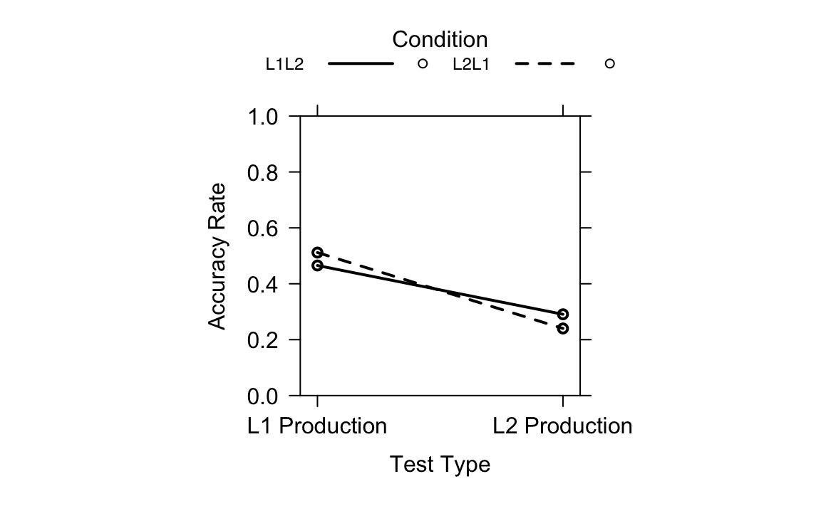
Figure 19.5 shows the interaction between Test Type and Learning Condition on accuracy rates, based on the generalized linear mixed-effects model (fit1.1). It is an effect plot generated with the allEffects() function. The solid line represents the L1 to L2 learning condition; the dotted line represents the L2 to L1 learning condition. The y-axis represents accuracy rates on both the L1 and L2 production tests. The x-axis represents the two test types. We can see that the accuracy rates differ across Test Types and Learning Conditions, with a clear interaction between the two: The non-parallel lines indicate that the effect of one variable changes depends on the level of the other variable. The distance between the two lines is relatively small at each test type, which reflects the results that revealed no significant difference in learning effects between L2 to L1 learning and L1 to L2 learning.
Generally, Terai, Yamashita & Pasich (2021) used base R plots in their original code. While there is nothing wrong with that, one could also use {ggplot2}, which provides many options to customise the plot. Also, it makes it easy to see what is plotted and how specific elements are modified, which can contribute to the reproducibility of the code. If you want to learn more about using {ggplot2}, check out Chapter 10.
19.5.2 Effects of Learning Directions and L2 Proficiency (RQ2)
Terai, Yamashita & Pasich (2021) hypothesized that the effectiveness of learning direction or word pairs might be dependent on the learners’ proficiency in English. In other words, lower-proficiency learners might benefit more from practicing in the L2 -> L1 direction, whilst higher-proficiency learners might benefit more from the L1 -> L2 direction.
To answer and test this question, the authors once again fit two separate generalized linear mixed models (GLMMs) for the L1 and L2 production tests. Before we work through the authors’ code step-by-step, we need to know what we are working with here: Our outcome variable is the accuracy on production tests and our predictor variables are the learning direction (L1 -> L2 vs. L2 -> L1) and participants’ vocabulary size (which is used as a proxy for English proficiency in this study). The random effects are Participant ID and Item ID so that the model can account for individual differences across participants and the property of individual vocabulary items.
19.5.2.1 L1 Production test
We begin by focusing only on the L1 production data. In the script they provided, the authors loaded the data again for this part and stored it as another object. However, we will continue to use dat to reproduce the code, instead. The authors used the function filter(), which only keeps the rows for the L1 Production test. This data is filtered because, while each participant took both L1 and L2 production tests, the authors found different patterns for both test types, which is why they chose to analyze them separately (Terai, Yamashita & Pasich 2021: 1126). This is the part where participants of the study had to produce the L1 (Japanese) word when shown the L2 (English) word.
dat.L1 <- filter(dat, Test == "L1 Production")Next, the learning directions (Condition) were converted to a factor. Terai, Yamashita & Pasich (2021) converted the categories (L1 -> L2 vs. L2 -> L1) into two factor levels so that R treats it as a categorical binary variable.
# Setting Condition (Learning direction) as a factor

dat.L1$Condition <- as.factor(dat.L1$Condition)
Here, too, the authors make use of contrast coding once more and standardised vocabulary scores:
c <- contr.treatment(2)
my.coding <- matrix(rep(1/2, 2, ncol = 1))
my.simple <- c-my.coding

contrasts(dat.L1$Condition) <- my.simple

dat.L1$s.vocab <- scale(dat.L1$Vocab)
19.5.2.2 Model without interaction
This model without interaction assumes that learning direction and L2 proficiency each have independent effects on test accuracy.
fit2 <- glmer(Answer ~ s.vocab + Condition +
(1|ID) + (1|ItemID),
family = binomial,
data = dat.L1,
glmerControl(optimizer = "bobyqa"))
summary(fit2)- 1
- The model formula includes main effects of learning condition and proficiency plus their interaction.
- 2
- The model formula also includes random intercepts for participants and items (to account for repeated measures).
- 3
- This is necessary because our outcome is binary (correct/incorrect).
Generalized linear mixed model fit by maximum likelihood (Laplace
  Approximation) [glmerMod]
 Family: binomial  ( logit )
Formula: Answer ~ s.vocab + Condition + (1 | ID) + (1 | ItemID)
   Data: dat.L1
Control: glmerControl(optimizer = "bobyqa")

      AIC       BIC    logLik -2*log(L)  df.resid
   1316.3    1341.2    -653.1    1306.3      1070

Scaled residuals:
    Min      1Q  Median      3Q     Max
-2.7382 -0.7161 -0.2849  0.7304  3.1811

Random effects:
 Groups Name        Variance Std.Dev.
 ItemID (Intercept) 0.9085   0.9531
 ID     (Intercept) 0.8452   0.9194
Number of obs: 1075, groups:  ItemID, 40; ID, 28

Fixed effects:
            Estimate Std. Error z value Pr(>|z|)
(Intercept)  -0.0468     0.2409  -0.194    0.846
s.vocab       0.1047     0.1846   0.567    0.571
Condition2    0.1874     0.1406   1.333    0.183

Correlation of Fixed Effects:
           (Intr) s.vocb
s.vocab    -0.025
Condition2  0.002  0.006
Further, Terai, Yamashita & Pasich (2021) computed the model’s AIC.
AIC(fit2) [1] 1316.26The model predicts the probability of a correct response (Answer). The random intercepts (1|ID) and (1|ItemID) account for individual differences between participants and for the unique difficulty of individual vocabulary items. The summary output of this model without interaction shows that s.vocab is not a significant predictor of retrieval accuracy with p = .57, which suggests that English proficiency by itself does not make a statistically significant contribution to the prediction of participants’ L1 Production accuracy. The model also suggests that the test Condition does not make a statistically significant contribution to the predictive accuracy of the model (p = .18), meaning that learning direction alone also does not explain differences. So, if we look at each predictor separately, there seems to be no clear effect.
19.5.2.3 Model with Interaction
What if English proficiency only matters in one of the two learning directions? To figure this out, Terai, Yamashita & Pasich (2021) added an interaction term to the model: s.vocab * Condition.
fit2.1 <- glmer(Answer ~ s.vocab * Condition + (1|ID) + (1|ItemID),
              family = binomial,
              data = dat.L1,
              glmerControl(optimizer = "bobyqa"))

summary(fit2.1)
Generalized linear mixed model fit by maximum likelihood (Laplace
Approximation) [glmerMod]
Family: binomial ( logit )
Formula: Answer ~ s.vocab * Condition + (1 | ID) + (1 | ItemID)
Data: dat.L1
Control: glmerControl(optimizer = "bobyqa")
AIC BIC logLik -2*log(L) df.resid
1311.6 1341.4 -649.8 1299.6 1069
Scaled residuals:
Min 1Q Median 3Q Max
-3.3577 -0.7070 -0.2723 0.7294 3.0368
Random effects:
Groups Name Variance Std.Dev.
ItemID (Intercept) 0.9314 0.9651
ID (Intercept) 0.8583 0.9265
Number of obs: 1075, groups: ItemID, 40; ID, 28
Fixed effects:
Estimate Std. Error z value Pr(>|z|)
(Intercept) -0.04872 0.24313 -0.200 0.84117
s.vocab 0.10336 0.18596 0.556 0.57834
Condition2 0.18358 0.14125 1.300 0.19368
s.vocab:Condition2 -0.36734 0.14148 -2.596 0.00942 **
---
Signif. codes: 0 '***' 0.001 '**' 0.01 '*' 0.05 '.' 0.1 ' ' 1
Correlation of Fixed Effects:
(Intr) s.vocb Cndtn2
s.vocab -0.026
Condition2 0.000 0.001
s.vcb:Cndt2 0.001 -0.003 0.006confint(fit2.1) 2.5 % 97.5 %
.sig01 0.73079922 1.28729202
.sig02 0.67541363 1.29848739
(Intercept) -0.53714956 0.43908234
s.vocab -0.27397898 0.48470670
Condition2 -0.09542877 0.46366465
s.vocab:Condition2 -0.64903456 -0.08897167AIC(fit2.1)[1] 1311.563As Terai, Yamashita & Pasich (2021) stated in their paper, the interaction of Learning Condition and Vocabulary Size is significant with a coefficient estimate of about -0.37, SE = 0.141, z = -2.596, p = .009, which means that the effect of vocabulary proficiency depends on the learning direction.
19.5.2.4 Visualization
Visualizing model predictions is a very useful way to better understand complex models like this one. Terai, Yamashita & Pasich (2021) visualized the model fit2.1 using the following base R plot.
plot(allEffects(fit2.1), multiline = T, ci.style = "bands",
    xlab = "Vocabulary Size", ylab = "Accuracy Rate",
    main = "", lty = c(1, 2),
    rescale.axis = F, ylim = c(0, 1), colors = "black", asp = 1)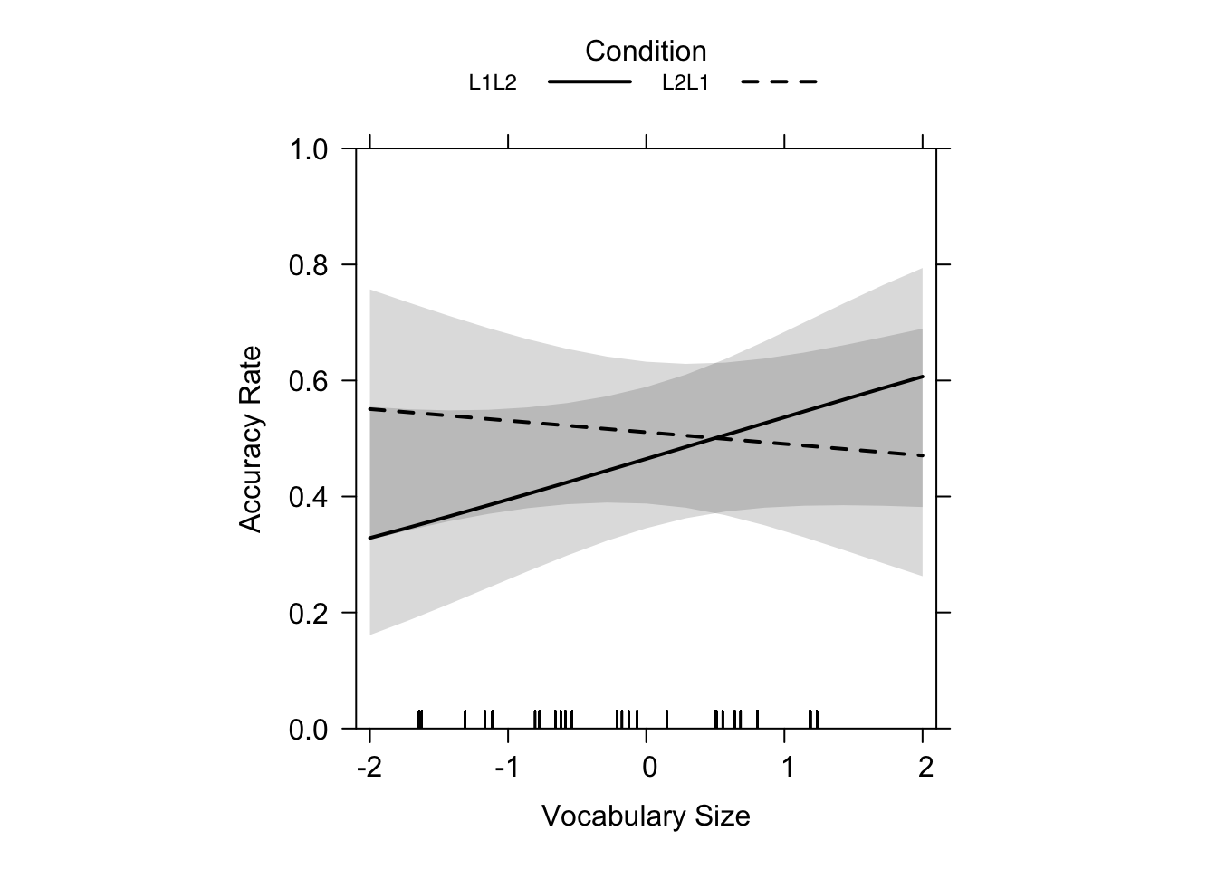
Figure 19.6 shows a solid line representing the L1 -> L2 learning condition, and a dotted line representing the L2 -> L1 learning condition. The y-axis shows L1 production accuracy rates of the test, and the x-axis the scaled scores of the vocabulary size tests (Terai, Yamashita & Pasich 2021: 1128). Looking at Figure 19.6 you can see a nearly flat line for L2 -> L1 and a positive, steeper line for L1 -> L2 which cross at intermediate proficiency (~5.419 as reported in the paper, p. 1127). The crossover point at ~5.419 suggests that for learners in the L1 -> L2 direction a score of over ~5.419 on the test for vocabulary size was more beneficial than for L2 -> L1 learners. The fact that the line for L2 -> L1 learning is nearly flat shows that proficiency in L2 did not have a big influence. Basically, the plot tells us that, for lower proficiency learners, L2 -> L1 is better, and for higher proficiency learners, L1 -> L2 is more beneficial (Terai, Yamashita & Pasich 2021: 1128).
19.5.2.5 L2 Production Test
Terai, Yamashita & Pasich (2021) repeated all the same steps for the L2 production test, now predicting accuracy for when the participants had to produce English words after learning Japanese-English pairs.
# Filtering the data we need
dat.L2 <- filter(dat, Test == "L2 Production")

# Setting Condition as factors
dat.L2$Condition <- as.factor(dat.L2$Condition)

c <- contr.treatment(2)
my.coding <- matrix(rep(1/2, 2, ncol = 1))
my.simple <- c-my.coding

contrasts(dat.L2$Condition) <- my.simple

# Scaling Vocab scores
dat.L2$s.vocab <- scale(dat.L2$Vocab)
# Model without interaction
fit3 <- glmer(Answer ~ s.vocab+Condition + (1|ID) + (1|ItemID),
family = binomial,
data = dat.L2,
glmerControl(optimizer = "bobyqa"))
summary(fit3)Generalized linear mixed model fit by maximum likelihood (Laplace
Approximation) [glmerMod]
Family: binomial ( logit )
Formula: Answer ~ s.vocab + Condition + (1 | ID) + (1 | ItemID)
Data: dat.L2
Control: glmerControl(optimizer = "bobyqa")
AIC BIC logLik -2*log(L) df.resid
1146.5 1171.4 -568.3 1136.5 1070
Scaled residuals:
Min 1Q Median 3Q Max
-2.2217 -0.5586 -0.3314 0.6289 5.0300
Random effects:
Groups Name Variance Std.Dev.
ItemID (Intercept) 1.5602 1.249
ID (Intercept) 0.8818 0.939
Number of obs: 1075, groups: ItemID, 40; ID, 28
Fixed effects:
Estimate Std. Error z value Pr(>|z|)
(Intercept) -1.1134 0.2799 -3.978 6.95e-05 ***
s.vocab 0.2293 0.1913 1.199 0.2306
Condition2 -0.2759 0.1538 -1.793 0.0729 .
---
Signif. codes: 0 '***' 0.001 '**' 0.01 '*' 0.05 '.' 0.1 ' ' 1
Correlation of Fixed Effects:
(Intr) s.vocb
s.vocab -0.037
Condition2 0.017 -0.001AIC(fit3)[1] 1146.519# Model with interaction
fit3.1 <- glmer(Answer ~ s.vocab * Condition + (1|ID) + (1|ItemID),
family = binomial,
data = dat.L2,
glmerControl(optimizer = "bobyqa"))
summary(fit3.1)Generalized linear mixed model fit by maximum likelihood (Laplace
Approximation) [glmerMod]
Family: binomial ( logit )
Formula: Answer ~ s.vocab * Condition + (1 | ID) + (1 | ItemID)
Data: dat.L2
Control: glmerControl(optimizer = "bobyqa")
AIC BIC logLik -2*log(L) df.resid
1145.3 1175.2 -566.7 1133.3 1069
Scaled residuals:
Min 1Q Median 3Q Max
-2.6092 -0.5624 -0.3263 0.6291 4.8839
Random effects:
Groups Name Variance Std.Dev.
ItemID (Intercept) 1.5769 1.2557
ID (Intercept) 0.8932 0.9451
Number of obs: 1075, groups: ItemID, 40; ID, 28
Fixed effects:
Estimate Std. Error z value Pr(>|z|)
(Intercept) -1.1196 0.2815 -3.978 6.96e-05 ***
s.vocab 0.2270 0.1925 1.179 0.2382
Condition2 -0.2623 0.1544 -1.699 0.0893 .
s.vocab:Condition2 -0.2780 0.1536 -1.809 0.0704 .
---
Signif. codes: 0 '***' 0.001 '**' 0.01 '*' 0.05 '.' 0.1 ' ' 1
Correlation of Fixed Effects:
(Intr) s.vocb Cndtn2
s.vocab -0.037
Condition2 0.014 0.012
s.vcb:Cndt2 0.019 0.003 -0.041confint(fit3.1) 2.5 % 97.5 %
.sig01 0.9458318 1.69373065
.sig02 0.6790647 1.33794127
(Intercept) -1.6989047 -0.56606911
s.vocab -0.1625726 0.62507709
Condition2 -0.5716568 0.04442562
s.vocab:Condition2 -0.5861211 0.02636997AIC(fit3.1)[1] 1145.316As for the first research question, the authors calculated AICs for both versions of the model, with and without interaction. We can see that the model with interaction has a lower AIC (1145.32) than the one without interaction (1146.52), which –as we remember– means that the model with the interaction is a better fit. Now, taking a look at the output of the summary() function, we see that the Vocabulary Size coefficient estimate is -0.227 (SE = 0.193, z = 1.179, p = .238). Our p-value is greater than 0.05, which means the effect is not statistically significant and proficiency alone does predict accuracy on the L2 production test. We see something nearly identical for the Learning condition with an estimate of -0.262 (SE = 0.154, z = -1.699, p = 0.089). This means that the performance is not predicted to significantly differ between the two learning directions. In a final step, the interaction term s.vocab * Condition was considered, which was also not statistically significant (β = -0.278, SE = 0.154, z = -1.810, p = .070).
19.5.2.6 Visualization
plot(allEffects(fit3.1), multiline = T, ci.style = "bands", xlab = "Vocabulary Size", ylab = "Accuracy Rate",
       main = "", lty = c(1, 2), rescale.axis = F, ylim = c(0, 1), colors = "black", asp = 1)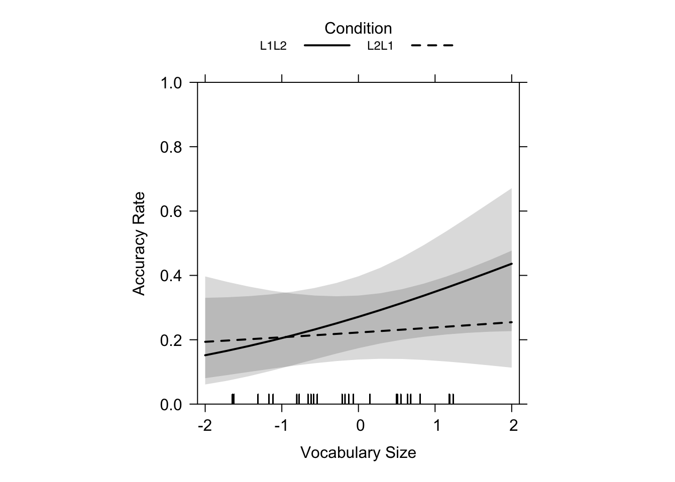
Just as the summary statistics of the model above suggested, Figure 19.7 shows that, while there was no significance of the results for learning direction or L2 proficiency, the trend bears similartiy to the results of our L1 production test (flatter L2 -> L1 slope, steeper L1 -> L2 slope). So, for lower-proficiency learners, L2 -> L1 leads to higher performance than L1 -> L2 learning. Furthermore, the authors explained that L2 -> L1 learning is much less influenced by L2 proficiency (Terai, Yamashita & Pasich 2021: 1128), which is clearly illustrated by the nearly flat dashed line in the graphs.
19.5.3 Interpretation & Take-home message
Generally, for the L1 production test, Terai, Yamashita & Pasich (2021)’s results showed that lower-proficiency learners benefited more from the L2 -> L1 learning direction, while higher-proficiency learners benefited more from the L1 -> L2 learning direction. For the L2 production test, a similar trend was observed, but it was not statistically significant, which calls for replication and further research. Overall, vocabulary proficiency shapes how effectively retrieval works: the optimal learning direction is not a one-size-fits-all matter, but may rather be dependent on learner proficiency. However, it is also worth highlighting that only a single language pair was tested in this study. Assuming that the above-mentioned results are generalisable L1-L2 effects may be a bit far-fetched.
19.5.4 Checking multicollinearity
Now, before interpreting these results too confidently, one should also check whether the predictors are highly correlated with one another, which would be a problem called multicollinearity (see Section 13.8) that might affect the results of our GLMMs.
Why does this matter? If the predictors are very strongly correlated, the model might have trouble to keep apart their unique contributions. It might then inflate standard errors and thus make estimates unreliable (Pennsylvania State University 2018).
A common diagnostic here is the Variance Inflation Factor (VIF). A VIF close to 1 means predictors are not collinear. Here are some rules: VIF = 1: perfect independence, VIF > 5: potential concern, VIF > 10: serious multicollinearity (Pennsylvania State University 2018).
19.5.4.1 Calculating VIFs for the Models
Terai, Yamashita & Pasich (2021) used a helper function vif.mer() to calculate VIFs for mixed models, which can be directly imported from GitHub using the source() function.
source("https://raw.githubusercontent.com/aufrank/R-hacks/master/mer-utils.R")

vif.mer(fit1.1)
Test2 Condition2 Test2:Condition2
1.001121 1.004295 1.004777 vif.mer(fit2.1) s.vocab Condition2 s.vocab:Condition2
1.000008 1.000044 1.000049 vif.mer(fit3.1) s.vocab Condition2 s.vocab:Condition2
1.000152 1.001814 1.001678 All the VIF values are obviously quite close to 1. This means that the predictors (s.vocab, Condition, and their interaction) are not correlated with each other in problematic ways. We can therefore be confident that the estimates of the interaction effects that were observed in the GLMMS are not due to multicollinearity.
19.6 Conclusion
You are now familiar with the interpretation of generalized linear mixed models! You have learned how to fit them, interpret their main effects and interactions, as well as checking for multicollinearity using the VIF measure. GLMMs are powerful tools for predicting binary outcomes such as true-false accuracy measures. They allow us to account for repeated measures across participants and items such as we encountered in this study by Terai, Yamashita & Pasich (2021). It is completely normal that at times GLMMs can feel intimidating: coding contrasts and interpreting the outcomes are not always straightforward. But there is always a solution. The insights we can gain from a nicely fitted model make all this effort worthwhile.
Owing to the fact that Terai, Yamashita & Pasich (2021) published their dataset and R code along with the publication, we were able to reproduce their findings and gain hands-on experience with modeling. This chapter does not include the reproduction and explanation of every part of the code that the authors shared, as we focused on the analyses discussed in Terai, Yamashita & Pasich (2021). In the reproduced code, we only changed minor things, like not reloading the same dataset several times under a different name. This sort of project not only helps with our understanding of the study, but it also sharpens our skills as future SLA researchers.
NoteHow to cite this chapter
This is a case study chapter of the web version of the textbook “Data Analysis for the Language Sciences: A very gentle introduction to statistics and data visualisation in R” by Elen Le Foll.
Please cite the current version of this chapter as:
Boxleitner, Hannah and Beyhan Aliy. 2025. Learning Direction Effects in Retrieval Practice on EFL Vocabulary Learning. In Elen Le Foll (Ed.), Data Analysis for the Language Sciences: A very gentle introduction to statistics and data visualisation in R. Open Educational Resource. https://elenlefoll.github.io/RstatsTextbook/ (accessed DATE).
References
[1] S. Amano and T. Kondo. Nihongo-no-Goitokusei Hindo [Lexical properties of Japanese: Frequency]. Sanseido, 2000.
[2] M. Barlaz. Contrast coding in R. 2022. https://marissabarlaz.github.io/portfolio/contrastcoding/#contrast-coding.
[3] B. M. Bolker. “13 Linear and generalized linear mixed models”. In: Ecological Statistics: Contemporary theory and application. Ed. by G. A. Fox, S. Negrete-Yankelevich and V. J. Sosa. Oxford Academic, 2015. DOI: 10.1093/acprof:oso/9780199672547.003.0014.
[4] J. M. Chambers and T. J. Hastie. Statistical models in S. New York: Routledge, 1992.
[5] S. Parajuli. Chapter 7 Skewness and Kurtosis. 2023. https://bookdown.org/subashparajuli/quant-r/skewness-and-kurtosis.html.
[6] Pennsylvania State University. 10.7 - Detecting Multicollinearity Using Variance Inflation Factors | STAT 462. 2018. https://online.stat.psu.edu/stat462/node/180/.
[7] M. Terai, J. Yamashita, and K. E. Pasich. “Effects of Learning Direction in Retrival Practice on EFL Vocabulary Learning”. In: Studies in Second Language Acquisition 43.5 (2021), pp. 1116-1137. DOI: https://doi.org/10.1017/S0272263121000346.
Package references
[1] D. Bates, M. Mächler, B. Bolker, et al. “Fitting Linear Mixed-Effects Models Using lme4”. In: Journal of Statistical Software 67.1 (2015), pp. 1-48. DOI: 10.18637/jss.v067.i01.
[2] D. Bates, M. Maechler, B. Bolker, et al. lme4: Linear Mixed-Effects Models using Eigen and S4. R package version 1.1-37. 2025. https://github.com/lme4/lme4/.
[3] D. Bates, M. Maechler, and M. Jagan. Matrix: Sparse and Dense Matrix Classes and Methods. R package version 1.7-3. 2025. https://Matrix.R-forge.R-project.org.
[4] C. Boettiger. knitcitations: Citations for Knitr Markdown Files. R package version 1.0.12. 2021. https://github.com/cboettig/knitcitations.
[5] P. Breheny and W. Burchett. visreg: Visualization of Regression Models. R package version 2.7.0. 2020. http://pbreheny.github.io/visreg.
[6] P. Breheny and W. Burchett. “Visualization of Regression Models Using visreg”. In: The R Journal 9.2 (2017), pp. 56-71.
[7] G. Csárdi, J. Hester, H. Wickham, et al. remotes: R Package Installation from Remote Repositories, Including GitHub. R package version 2.5.0. 2024. https://remotes.r-lib.org.
[8] H. De Rosario-Martinez. phia: Post-Hoc Interaction Analysis. R package version 0.3-2. 2025. https://github.com/heliosdrm/phia.
[9] A. Eklund and J. Trimble. beeswarm: The Bee Swarm Plot, an Alternative to Stripchart. R package version 0.4.0. 2021. https://github.com/aroneklund/beeswarm.
[10] S. A. file. paletteer: Comprehensive Collection of Color Palettes. R package version 1.6.0. 2024. https://github.com/EmilHvitfeldt/paletteer.
[11] J. Fox. “Effect Displays in R for Generalised Linear Models”. In: Journal of Statistical Software 8.15 (2003), pp. 1-27. DOI: 10.18637/jss.v008.i15.
[12] J. Fox and J. Hong. “Effect Displays in R for Multinomial and Proportional-Odds Logit Models: Extensions to the effects Package”. In: Journal of Statistical Software 32.1 (2009), pp. 1-24. DOI: 10.18637/jss.v032.i01.
[13] J. Fox and S. Weisberg. An R Companion to Applied Regression. Third. Thousand Oaks CA: Sage, 2019. https://www.john-fox.ca/Companion/.
[14] J. Fox and S. Weisberg. An R Companion to Applied Regression. 3rd. Thousand Oaks CA: Sage, 2019. https://socialsciences.mcmaster.ca/jfox/Books/Companion/index.html.
[15] J. Fox and S. Weisberg. “Visualizing Fit and Lack of Fit in Complex Regression Models with Predictor Effect Plots and Partial Residuals”. In: Journal of Statistical Software 87.9 (2018), pp. 1-27. DOI: 10.18637/jss.v087.i09.
[16] J. Fox, S. Weisberg, and B. Price. car: Companion to Applied Regression. R package version 3.1-3. 2024. https://r-forge.r-project.org/projects/car/.
[17] J. Fox, S. Weisberg, and B. Price. carData: Companion to Applied Regression Data Sets. R package version 3.0-5. 2022. https://r-forge.r-project.org/projects/car/.
[18] J. Fox, S. Weisberg, B. Price, et al. effects: Effect Displays for Linear, Generalized Linear, and Other Models. R package version 4.2-2. 2022. https://www.r-project.org.
[19] G. Grolemund and H. Wickham. “Dates and Times Made Easy with lubridate”. In: Journal of Statistical Software 40.3 (2011), pp. 1-25. https://www.jstatsoft.org/v40/i03/.
[20] L. Komsta and F. Novomestky. moments: Moments, Cumulants, Skewness, Kurtosis and Related Tests. R package version 0.14.1. 2022. https://www.r-project.org.
[21] R. V. Lenth. emmeans: Estimated Marginal Means, aka Least-Squares Means. R package version 1.11.1. 2025. https://rvlenth.github.io/emmeans/.
[22] K. Müller. here: A Simpler Way to Find Your Files. R package version 1.0.1. 2020. https://here.r-lib.org/.
[23] K. Müller and H. Wickham. tibble: Simple Data Frames. R package version 3.3.0. 2025. https://tibble.tidyverse.org/.
[24] R Core Team. R: A Language and Environment for Statistical Computing. R Foundation for Statistical Computing. Vienna, Austria, 2025. https://www.R-project.org/.
[25] W. Revelle. psych: Procedures for Psychological, Psychometric, and Personality Research. R package version 2.5.3. 2025. https://personality-project.org/r/psych/.
[26] V. Spinu, G. Grolemund, and H. Wickham. lubridate: Make Dealing with Dates a Little Easier. R package version 1.9.4. 2024. https://lubridate.tidyverse.org.
[27] H. Wickham. forcats: Tools for Working with Categorical Variables (Factors). R package version 1.0.1. 2025. https://forcats.tidyverse.org/.
[28] H. Wickham. ggplot2: Elegant Graphics for Data Analysis. Springer-Verlag New York, 2016. ISBN: 978-3-319-24277-4. https://ggplot2.tidyverse.org.
[29] H. Wickham. stringr: Simple, Consistent Wrappers for Common String Operations. R package version 1.6.0. 2025. https://stringr.tidyverse.org.
[30] H. Wickham. tidyverse: Easily Install and Load the Tidyverse. R package version 2.0.0. 2023. https://tidyverse.tidyverse.org.
[31] H. Wickham, M. Averick, J. Bryan, et al. “Welcome to the tidyverse”. In: Journal of Open Source Software 4.43 (2019), p. 1686. DOI: 10.21105/joss.01686.
[32] H. Wickham, W. Chang, L. Henry, et al. ggplot2: Create Elegant Data Visualisations Using the Grammar of Graphics. R package version 4.0.1. 2025. https://ggplot2.tidyverse.org.
[33] H. Wickham, R. François, L. Henry, et al. dplyr: A Grammar of Data Manipulation. R package version 1.1.4. 2023. https://dplyr.tidyverse.org.
[34] H. Wickham and L. Henry. purrr: Functional Programming Tools. R package version 1.2.0. 2025. https://purrr.tidyverse.org/.
[35] H. Wickham, J. Hester, and J. Bryan. readr: Read Rectangular Text Data. R package version 2.1.5. 2024. https://readr.tidyverse.org.
[36] H. Wickham, D. Vaughan, and M. Girlich. tidyr: Tidy Messy Data. R package version 1.3.1. 2024. https://tidyr.tidyverse.org.
[37] Y. Xie. Dynamic Documents with R and knitr. 2nd. ISBN 978-1498716963. Boca Raton, Florida: Chapman and Hall/CRC, 2015. https://yihui.org/knitr/.
[38] Y. Xie. “knitr: A Comprehensive Tool for Reproducible Research in R”. In: Implementing Reproducible Computational Research. Ed. by V. Stodden, F. Leisch and R. D. Peng. ISBN 978-1466561595. Chapman and Hall/CRC, 2014.
[39] Y. Xie. knitr: A General-Purpose Package for Dynamic Report Generation in R. R package version 1.50. 2025. https://yihui.org/knitr/.
[40] H. Zhu. kableExtra: Construct Complex Table with kable and Pipe Syntax. R package version 1.4.0. 2024. http://haozhu233.github.io/kableExtra/.