17  The gRammaticalization of ‘perdón’ in Spanish varieties

About the author of this chapter

Dela (Fatemeh) Modir Dehghan is a Master’s student in linguistics at the University of Cologne in Germany. Originally from Iran, she completed her Bachelor’s degree in 2023 in English linguistics and translation at Alborz University.She is particularly interested in corpus-based explorations of language and aims to investigate how language changes over time using real-world data. She submitted an earlier version of this chapter as a term paper as part of Dr. Le Foll’s M.A. seminar on Statistics and Data Visualisation in R.

This chapter will guide you through the steps to reproduce the results of a published corpus linguistics study (Jansegers, Melis & Arrington 2024) using R. It will walk you through how to:

• Download and load the original dataset provided by Jansegers, Melis & Arrington (2024) into R
• Understand the structure and the linguistic variables of the dataset (Spanish variety, offense type, and apology form)
• Wrangle the data to categorize perdón, disculpa, and lo siento by pragmatic function
• Analyze the use of perdón as a discourse marker in Mexican and Peninsular Spanish
• Reproduce the key descriptive statistics and test results reported in Jansegers, Melis & Arrington (2024).
• Compare the reproduced values (e.g., frequency counts, significance tests) with those reported in the original study
• Visualize trends across varieties and offense types using {ggplot2} to support the interpretation of the findings.

Whether you are new to R or seeking to sharpen your analytical skills, this chapter provides a guided, reproducible introduction to data-driven linguistic analysis using Spanish apology markers as a case study.

17.1 Introducing the study

In this chapter, we reproduce the results of a corpus linguistics study (Jansegers, Melis & Arrington 2024), which investigates the grammaticalization of the Spanish apology marker perdón in two regional varieties: Mexican and Peninsular Spanish. Grammaticalization refers to the historical process by which lexical items such as verbs or nouns evolve into grammatical or discourse-related elements (Hopper & Traugott 2003; Heine & Kuteva 2002). In this case, the verb perdonar (‘to pardon’) has undergone semantic and functional shifts, becoming the discourse marker perdón, particularly in the context of low-imposition offenses.

The original study (Jansegers, Melis & Arrington 2024) analyzes corpus data to explore how apology markers (perdón, lo siento, disculpa) vary according to factors such as offense type, speaker responsibility, and Spanish variety. Their methodology draws on frameworks from grammaticalization theory (Hopper & Traugott 2003) and politeness theory (Brown & Levinson 1987).

Our goal is to reproduce the analyses of Jansegers, Melis & Arrington (2024) using the same dataset and statistical procedures, and visualizations in R. This will allow us to compare our outputs to those reported in the original study and assess the consistency of results across offense types and regional varieties.

This reproduction focuses on the following research question:

• Does perdón function differently in Mexican and Peninsular Spanish?

17.2 Retrieving the data

We begin by retrieving the original dataset used in the study by Jansegers, Melis & Arrington (2024). The researchers compiled corpus data from two distinct varieties of Spanish:

• Mexican Spanish
• Peninsular Spanish

These datasets are made up of real-life language interactions, including transcripts of conversations, online discussions, and formal writing. Each part of the corpus has been carefully annotated to highlight apology phrases like perdón, disculpa, and lo siento showing how they are used in different contexts.

In their open-access publication in Languages, the authors included the following Data Availability Statement (Jansegers, Melis & Arrington 2024: 19):

Data Availability Statement
The research data of this study is available in TROLLing. Jansegers, Marlies; Melis, Chantal; Arrington Báez, Jennie Elenor, 2023, Replication Data for: Diverging grammaticalization patterns across Spanish varieties: the case of perdón in Mexican and Peninsular Spanish, https://doi.org/10.18710/IEXVVN (accessed on 1 December 2023), DataverseNO.

To obtain the dataset, follow these straightforward steps:

• Follow the link to the data repository:
  https://doi.org/10.18710/IEXVVN
• Locate the dataset:
  Locate the dataset file named Data_perdon_20231221.csv.
• Download the dataset:
  Save the CSV file (Data_perdon_20231221.csv) to your local project directory.

17.3 Preprocessing the data

To get started, you’ll want to load (and if necessary, first install) the R libraries that we will need for this reproduction project.

library(here) # Useful for file path management.
library(ggmosaic) # Visualizes relationships in data through mosaic plots in {ggplot2}.
library(kableExtra) # To display nice-looking tables.
library(skimr) # Provides summaries of dataset variables for quick insights into distributions and missing data.
library(tidyverse) # A collection of core data science packages, including {ggplot2} and {dplyr} for data visualisation, data wrangling, and data import.

Once the necessary packages are loaded, we can read in the dataset and check its contents. Note that the dataset is semi-colon separated.

# Import the dataset
data <- read.csv(here("B_CaseStudies", "Dela", "Data_perdon_20231221.csv"), sep = ";")

# Display the first few rows
head(data)

  variety  corpus      form           offense_type face_affected
1      MX PRESEEA disculpar inappropriate_behavior      positive
2      MX PRESEEA disculpar     lack_consideration      positive
3      MX PRESEEA disculpar      censored_language      positive
4      MX PRESEEA disculpar     temporal_territory      negative
5      MX PRESEEA disculpar           slips_tongue      positive
6      MX PRESEEA disculpar           slips_tongue      positive
  face_orientation
1          speaker
2           hearer
3          speaker
4           hearer
5          speaker
6          speaker

• The dataset is stored as a CSV file, so we use read.csv().
• sep = ";" ensures the correct delimiter is used (European-style CSVs).
• head(data) helps us quickly preview the dataset.

Now that we have imported the data , it’s crucial to understand the structure of the dataset to ensure all variables are correctly formatted.

# Check the structure of the dataset
str(data)

'data.frame':   769 obs. of  6 variables:
 $ variety         : chr  "MX" "MX" "MX" "MX" ...
 $ corpus          : chr  "PRESEEA" "PRESEEA" "PRESEEA" "PRESEEA" ...
 $ form            : chr  "disculpar" "disculpar" "disculpar" "disculpar" ...
 $ offense_type    : chr  "inappropriate_behavior" "lack_consideration" "censored_language" "temporal_territory" ...
 $ face_affected   : chr  "positive" "positive" "positive" "negative" ...
 $ face_orientation: chr  "speaker" "hearer" "speaker" "hearer" ...

In this step, we need to check for missing values before we start the analysis.

# Check for missing values
sum(is.na(data))

[1] 0

To further understand the dataset, let’s generate summary descriptive statistics.

# Get an overview of the dataset
skim(data)

Data summary

Name	data
Number of rows	769
Number of columns	6
_______________________
Column type frequency:
character	6
________________________
Group variables	None

Variable type: character

skim_variable	n_missing	complete_rate	min	max	empty	n_unique	whitespace
variety	0	1	2	2	0	2	0
corpus	0	1	3	10	0	9	0
form	0	1	6	9	0	4	0
offense_type	0	1	10	22	0	14	0
face_affected	0	1	8	8	0	2	0
face_orientation	0	1	6	7	0	2	0

📝 Quiz Time!

[Q1] When importing the dataset, why do we specify sep = ";" in read.csv()?

Because the CSV uses semicolons as the separator character
To automatically remove rows with missing values
To indicate that this dataset uses semicolons instead of decimal points
To convert columns contain texts into factors
To speed up the import of large datasets like this one

🐭 Click for a hint!

[Q2] What is the purpose of using skim(data) after importing the dataset?

To quickly summarize variable types, missing values, and distributions
To delete redundant columns automatically
To detect and replace missing values with averages
To visualize the data with {ggplot2}

🐭 Click for a hint!

17.4 Reviewing the variables

The dataset consists primarily of categorical variables, each of which represents a set of predefined categories. Understanding these variables and the levels that they can take is essential before beginning analysis:

• variety: Refers to the regional variety of Spanish in which the apology occurs.
  • Levels: MX (Mexican) and SP (Peninsular).
• corpus: Indicates the specific corpus or sub-corpus from which the example was drawn.
  • Levels: PRESEEA, CSCM, CHBC, CME, Ameresco, CORMA, VALESCO, C-ORAL-ROM, and CORLEC.
• form: The type of apology marker used in the utterance.
  • Levels: perdón, disculpar, perdonar, and lo siento
• offense_type: Categorizes the nature or source of the offense prompting the apology.
  • Levels: inappropriate_behavior, criticism_disagreement, obligation, damage_belongings, etc. (14 specific types in total)
• face_affected: Describes whose face (i.e., social identity or image) is being addressed or repaired by the apology.
  • Levels: positive, negative.
• face_orientation: Refers to whether the apology is oriented toward preserving the speaker’s own face or that of another.
  • Levels: speaker, hearer.

Since many of our variables are categorical (variety, form, offense_type, etc.), we convert them to factors to facilitate the analysis in R.

data_filtered <- data |>
  mutate(across(c(form, variety, offense_type, face_affected, face_orientation), factor))

Now that our dataset is well-structured, we can move forward to descriptive statistics and visualization Section 17.5.

17.5 Plotting the results

First, we take a look at frequency of the the different forms of apology markers across both Spanish varieties.

# Count frequency of apology markers
apology_counts <- data |>
  count(variety, form) |>
  arrange(desc(n))

apology_counts |> 
  kable()

variety	form	n
MX	perdón	299
SP	perdón	201
SP	perdonar	158
MX	disculpar	49
SP	lo siento	35
SP	disculpar	12
MX	perdonar	11
MX	lo siento	4

To better visualize the contrast, we also create a grouped bar chart.

ggplot(apology_counts, aes(x = form, 
                           y = n, 
                           fill = variety)) +
  geom_col(position = "dodge") +
  labs(
    title = "Frequency of Apology Markers by Spanish Variety",
    x = "Apology Marker",
    y = "Count",
    fill = "Variety"
  ) +
  theme_minimal()

Figure 17.1: Frequency of Apology Markers

This chart confirms the trends reported by Jansegers, Melis & Arrington (2024): perdón is the most frequent marker, especially in Mexican Spanish, while Peninsular Spanish shows a broader mix of forms. These findings align with politeness theory (Brown & Levinson 1987), which explains cultural variation in face strategies, and grammaticalization frameworks (Hopper & Traugott 2003; Heine & Kuteva 2002), which describe how frequent lexical items become discourse markers.

While Figure 17.1 earlier provided an overall frequency comparison of apology markers across Spanish varieties, mosaic plots allow for a more detailed visualization. To visualize how apology marker usage differs by Spanish variety, we use geom_mosaic() from the {ggmosaic} package. This plot shows the distribution of the different apology forms across Mexican and Peninsular Spanish, with bar widths reflecting the relative frequencies within each variety.

ggplot(data_filtered) +
  geom_mosaic(aes(x = product(variety), 
                  fill = form, 
                  weight = 1)) +
  labs(
    title = "Mosaic Plot: Apology Marker Distribution by Variety",
    x = "Spanish Variety",
    y = "Proportion of Apology Markers",
    fill = "Apology Marker"
  ) +
  theme_minimal()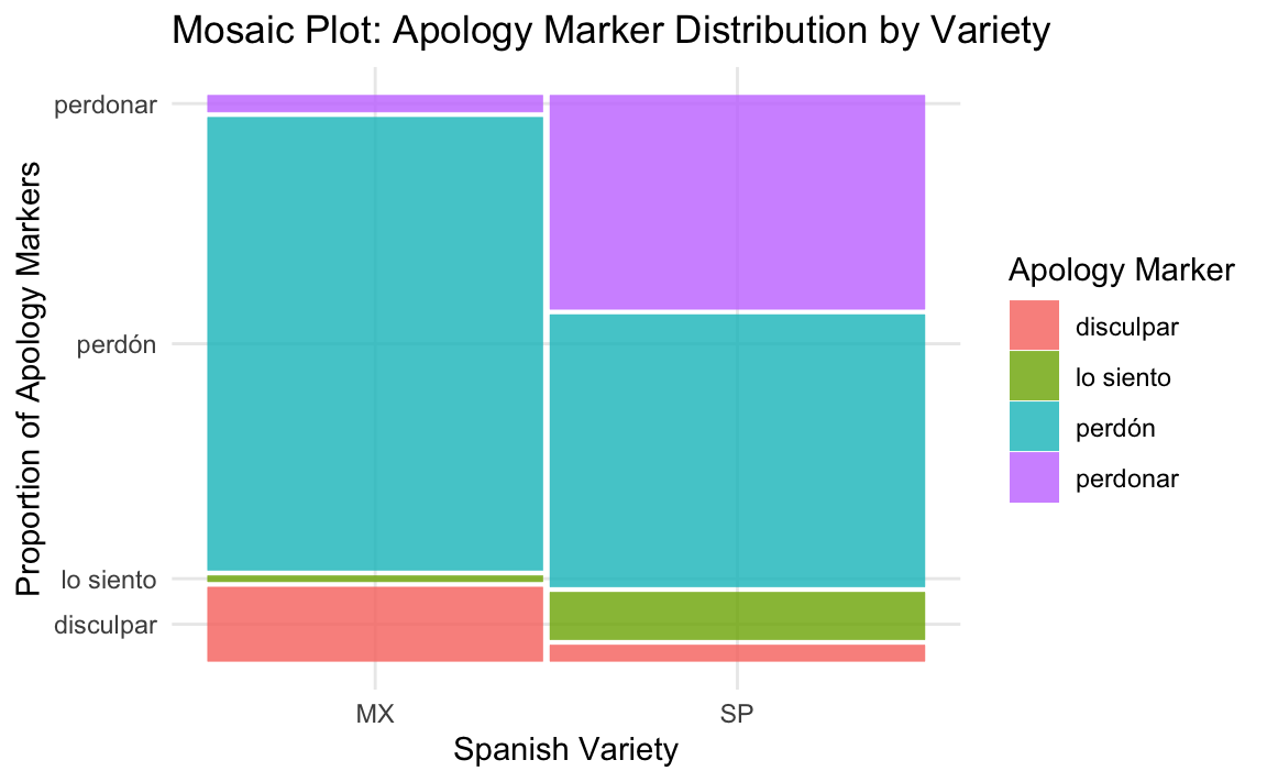

Figure 17.2: Mosaic Plot: Apology Marker Distribution by Variety

📝 Quiz Time!

[Q3] What does the height (length) of the bars represent in Figure 17.2?

The number of apology marker types across the two Spanish varieties
The relative frequency of each apology marker within each Spanish variety
The number of face-orientation contexts in both Mexican and Peninsular Spanish
The number of corpus observations in each Spanish variety

🐭 Click for a hint!

17.6 Reproducing the tables

In this section, we reproduce the main descriptive statistics from Jansegers, Melis & Arrington (2024) regarding the distribution of explicit apology markers across Spanish varieties and face orientations.

We begin by reconstructing the contingency table comparing Mexican and Peninsular Spanish in Table 17.1. We then break down the use of each form in relation to face-orientation contexts for both Mexican (Table 17.2) and Peninsular (Table 17.3) speakers. Frequencies and row-wise percentages are included to match the original analysis.

17.6.1 Shared methodology

All tables were generated using the following functions:

• count() to obtain for raw frequencies per combination of characteristics.
• proportions() × 100 for percentages within each group.
• paste0() to combine counts and percentages.
• pivot_wider() to reshape for display comparable to the original publication.
  • names_from = form uses the unique apology forms to create new columns.
  • values_from = n_pct fills those columns with the combined “count (percent)” strings.

We only varied the grouping/filtering depending on the table’s focus.

17.6.2 Apology forms by variety

To begin, we count the number of each apology form in Mexican and Peninsular Spanish, and then calculate row-wise percentages using group_by() and proportions() to show relative frequency across varieties.

apology_table <- data |>
  count(variety, form) |>
  group_by(variety) |>
  mutate(percentage = round(proportions(n) * 100, 0)) |>
  mutate(n_pct = paste0(n, " (", percentage, "%)")) |>
  select(variety, form, n_pct) |>
  pivot_wider(names_from = variety, values_from = n_pct)

apology_table |> 
  kable()

Table 17.1: Apology Marker Distribution by Variety

form	MX	SP
disculpar	49 (13%)	12 (3%)
lo siento	4 (1%)	35 (9%)
perdonar	11 (3%)	158 (39%)
perdón	299 (82%)	201 (50%)

Table 17.1 is a reproduction of Table 2 from Jansegers, Melis & Arrington (2024). The results show a clear preference for perdón in Mexico, while perdonar is more common in Spain. This contrast reflects broader regional differences in formality and apology strategies.

The percentages didn’t exactly match the original article due to rounding difference. While 49 / 363 equals 13.49%, R’s round() function rounds it down to 13%, whereas the original paper rounds it up to 14%.

This minor discrepancy affects only one cell in the table and does not impact the overall distribution pattern.

17.6.3 Conducting a Chi-square test

Building on the findings summarised in Table 17.1, we now test whether the observed differences in apology form usage between Mexican and Peninsular Spanish are statistically significant at an alpha level of 0.05. In line with the original study (Jansegers, Melis & Arrington 2024), we applied a Chi-square test to test this.

# Create a contingency table
apology_matrix <- table(data$variety, data$form)

# Run the Chi-square test
chisq.test(apology_matrix)

    Pearson's Chi-squared test

data:  apology_matrix
X-squared = 192.35, df = 3, p-value < 2.2e-16

The Chi-Square test that there is a statistically significant association between Spanish variety and apology marker (χ² = 192.35, df = 3, p < .001), matching the results in Jansegers, Melis & Arrington (2024).

17.6.4 Apology forms by face orientation (Mexico)

To produce Table 3 from Jansegers, Melis & Arrington (2024), we extend the procedure used to generate Table 17.1 by introducing a new composite variable, face_group, which merges face_orientation and face_affected into three analytically meaningful categories:

• Positive face S (speaker’s face affected),
• Negative face H (hearer’s negative face),
• Positive face H (hearer’s positive face).

These reflects the speaker vs. hearer face-threat distinctions used by Jansegers, Melis & Arrington (2024).

mexico_forms <- data |>
  filter(variety == "MX") |>
  mutate(face_group = case_when(
    face_orientation == "speaker" ~ "Positive face S",
    face_orientation == "hearer" & face_affected == "negative" ~ "Negative face H",
    face_orientation == "hearer" & face_affected == "positive" ~ "Positive face H"
  )) |>
  count(face_group, form) |>
  group_by(face_group) |>
  mutate(pct = round(100 * n / sum(n))) |>
  mutate(n_pct = paste0(n, " (", pct, "%)")) |>
  select(face_group, form, n_pct) |>
  pivot_wider(names_from = form, values_from = n_pct)

mexico_forms |> 
  kable()

Table 17.2: Apology Forms by Face Orientation (Mexico), Table 3

face_group	disculpar	lo siento	perdonar	perdón
Negative face H	22 (18%)	1 (1%)	6 (5%)	90 (76%)
Positive face H	12 (40%)	3 (10%)	2 (7%)	13 (43%)
Positive face S	15 (7%)	NA	3 (1%)	196 (92%)

Our output confirms the study’s finding that perdón is strongly favored when the speaker’s own face is at stake. All percentages and frequencies match those in the original study exactly, without rounding differences.

17.6.5 Apology forms by face orientation (Spain)

We recreate Table 4 from the original study by grouping the Peninsular Spanish data by face orientation and face affected.

spain_forms <- data |>
  filter(variety == "SP") |>
  mutate(face_group = case_when(
    face_orientation == "speaker" ~ "Positive face S",
    face_orientation == "hearer" & face_affected == "negative" ~ "Negative face H",
    face_orientation == "hearer" & face_affected == "positive" ~ "Positive face H"
  )) |>
  count(face_group, form) |>
  group_by(face_group) |>
  mutate(pct = round(100 * n / sum(n))) |>
  mutate(n_pct = paste0(n, " (", pct, "%)")) |>
  select(face_group, form, n_pct) |>
  pivot_wider(names_from = form, values_from = n_pct)

spain_forms |> 
  kable()

Table 17.3: Apology Forms by Face Orientation (Spain), Table 4

face_group	disculpar	lo siento	perdonar	perdón
Negative face H	7 (4%)	15 (9%)	88 (50%)	66 (38%)
Positive face H	1 (2%)	14 (22%)	39 (61%)	10 (16%)
Positive face S	4 (2%)	6 (4%)	31 (19%)	125 (75%)

The results match those reported in the original study (Jansegers, Melis & Arrington 2024): the verb perdonar is common in hearer-oriented contexts, while perdón appears more in speaker-oriented ones. The small discrepancies observed such as 36% instead of 37% for perdón under Negative face H, or 17% instead of 16% under Positive face H are limited to 1 percentage point and likely stem from rounding differences in the percentage calculations (see ?round()). These very minor differences do not affect the interpretation of the results.

Quiz Time!

📝 Let’s check your understanding of the data wrangling steps necessary to generate these tables!

[Q4] What does the paste0() function do?

It combines count values and percentages into a single vector.
It formats columns for easy export to Word.
It calculates percentages.
It combines two or more vectors into one and separates these vectors with the number 0.

🐭 Click for a hint!

[Q5] Why did we use pivot_wider() in our table generation steps?

To convert the long-format counts into a wide-format table with forms as columns.
To make the plot display the x-axis in alphabetical order.
To automatically rename the apology marker variables.
To filter out rows with zero frequency.

🐭 Click for a hint!

17.7 Conclusion

This project set out to reproduce the main findings of Jansegers, Melis & Arrington (2024), which explored the grammaticalization of perdón in Mexican and Peninsular Spanish. We were able to reproduce the findings of the original authors: in this corpus data, perdón is far more frequent in Mexican Spanish, while Peninsular Spanish speakers make use of a broader range of apology forms, including perdonar and lo siento. The frequency tables and percentage distributions that we reproduced from the author’s original data closely mirror those published in the original study.

Beyond reproducing the numerical results, we also matched the study’s visualizations using bar plots (Figure 17.1) and mosaic plots (Figure 17.2), which clearly show how apology strategies vary by variety and face orientation. These visuals help to illustrate the claim that perdón has undergone grammaticalization—especially in Mexican Spanish into a high-frequency discourse marker used to manage politeness.

Overall, the reproduction validates both the descriptive and statistical results of the original study, demonstrating how perdón’s usage reflects broader sociopragmatic and grammatical trends across Spanish varieties. Minor formatting or rounding differences aside, our results strongly align with the published findings and reinforce the value of data sharing in corpus-based linguistic research.

17.7.1 Suggestions for future research

While this project successfully reproduces and extends the findings of Jansegers, Melis & Arrington (2024), further studies could enrich the analysis by incorporating additional Spanish varieties beyond Mexico and Spain, or by examining sociolinguistic variables such as speaker age, gender, and social status (see, e.g., Hernández-Campoy & Conde-Silvestre 2012). Longitudinal research could also explore whether the grammaticalization of perdón continues to evolve over time.

📌 Implementing Citation Management with .bib in Quarto

To ensure standardized citation formatting, this project employs a BibTeX (.bib) file, referenced within the YAML metadata. The .bib file (e.g., final.bib) is specified under the bibliography field, allowing Quarto to format in-text citations and automatically generate a reference list.

Additionally, a Citation Style Language (CSL) file (apa.csl) is included to enforce APA-style referencing. This setup enables seamless integration of bibliographic data while maintaining consistency across the document.

In-text citations are implemented using the @key notation, which Quarto automatically resolves into properly formatted references during rendering.

For more information on how to insert bibliographic references in Quarto documents, see Section 14.9.

Packages used in this chapter

[1] H. Jeppson, H. Hofmann, and D. Cook. _ggmosaic: Mosaic Plots in the
ggplot2 Framework_. R package version 0.3.3. 2021.
<https://github.com/haleyjeppson/ggmosaic>.

[2] K. Müller and H. Wickham. _tibble: Simple Data Frames_. R package
version 3.2.1. 2023. <https://tibble.tidyverse.org>.

[3] B. Ripley. _nnet: Feed-Forward Neural Networks and Multinomial
Log-Linear Models_. R package version 7.3-20. 2025.
<http://www.stats.ox.ac.uk/pub/MASS4/>.

[4] V. Spinu, G. Grolemund, and H. Wickham. _lubridate: Make Dealing
with Dates a Little Easier_. R package version 1.9.3. 2023.
<https://lubridate.tidyverse.org>.

[5] E. Waring, M. Quinn, A. McNamara, et al. _skimr: Compact and
Flexible Summaries of Data_. R package version 2.1.5. 2022.
<https://docs.ropensci.org/skimr/>.

[6] H. Wickham. _forcats: Tools for Working with Categorical Variables
(Factors)_. R package version 1.0.0,
<https://github.com/tidyverse/forcats>. 2023.
<https://forcats.tidyverse.org>.

[7] H. Wickham. _tidyverse: Easily Install and Load the Tidyverse_. R
package version 2.0.0, <https://github.com/tidyverse/tidyverse>. 2023.
<https://tidyverse.tidyverse.org>.

[8] H. Wickham, W. Chang, L. Henry, et al. _ggplot2: Create Elegant
Data Visualisations Using the Grammar of Graphics_. R package version
3.5.1, <https://github.com/tidyverse/ggplot2>. 2024.
<https://ggplot2.tidyverse.org>.

[9] H. Wickham, R. François, L. Henry, et al. _dplyr: A Grammar of Data
Manipulation_. R package version 1.1.4. 2023.
<https://dplyr.tidyverse.org>.

[10] H. Wickham and L. Henry. _purrr: Functional Programming Tools_. R
package version 1.0.2. 2023. <https://purrr.tidyverse.org>.

[11] H. Wickham, J. Hester, and J. Bryan. _readr: Read Rectangular Text
Data_. R package version 2.1.5. 2024. <https://readr.tidyverse.org>.

[12] H. Wickham, D. Vaughan, and M. Girlich. _tidyr: Tidy Messy Data_.
R package version 1.3.1. 2024. <https://tidyr.tidyverse.org>.

References

[1] P. Brown and S. C. Levinson. Politeness: Some Universals in Language Usage. Cambridge University Press, 1987. https://www.cambridge.org/core/books/politeness-some-universals-in-language-usage/.

[2] B. Heine and T. Kuteva. World Lexicon of Grammaticalization. Cambridge University Press, 2002. https://doi.org/10.1017/CBO9780511613463.

[3] J. M. Hernández-Campoy and J. C. Conde-Silvestre. The Handbook of Historical Sociolinguistics. Wiley-Blackwell, 2012. https://doi.org/10.1017/S0047404515000688.

[4] P. Hopper and E. C. Traugott. Grammaticalization. Cambridge University Press, 2003. https://doi.org/10.1017/CBO9781139165525.

[5] M. Jansegers, E. Melis, and G. Arrington. “The Grammaticalization of Perdón in Spanish Varieties”. In: Journal of Pragmatics 192 (2024), pp. 15-32. https://doi.org/10.3390/languages9010013.

[6] E. C. Traugott and R. B. Dasher. Regularity in Semantic Change. Cambridge University Press, 2001. https://doi.org/10.1017/CBO9780511486500.

[7] H. Wickham. ggplot2: Elegant Graphics for Data Analysis. Springer, 2016. https://ggplot2-book.org/.

Brown, Penelope & Stephen C. Levinson. 1987. Politeness: Some universals in language usage. Cambridge University Press. https://www.cambridge.org/core/books/politeness-some-universals-in-language-usage/.

Heine, Bernd & Tania Kuteva. 2002. World lexicon of grammaticalization. Cambridge University Press. https://doi.org/10.1017/CBO9780511613463.

Hernández-Campoy, Juan Manuel & Juan Camilo Conde-Silvestre. 2012. The handbook of historical sociolinguistics. Wiley-Blackwell. https://doi.org/10.1017/S0047404515000688.

Hopper, Paul & Elizabeth Closs Traugott. 2003. Grammaticalization. Cambridge University Press. https://doi.org/10.1017/CBO9781139165525.

Jansegers, Marlies, Estela Melis & G. Arrington. 2024. The grammaticalization of perdón in spanish varieties. Journal of Pragmatics 192. 15–32. https://doi.org/10.3390/languages9010013.