Ch. 13: Tasks & Quizzes

TipYour turn!

The dataset from Dąbrowska (2019) includes a variable that we have not explored yet: ART. It stands for Author Recognition Test (Acheson, Wells & MacDonald 2008) and is a measure of print exposure to (almost exclusively Western, English-language) literature. Dąbrowska (2019: 9) explains the testing instrument and her motivation for including it in her battery of tests as follows:

The test consists of a list of 130 names, half of which are names of real authors. The participants’ task is to mark the names that they know to be those of published authors. To penalize guessing, the score is computed by subtracting the number of foils [wrong guesses] from the number of real authors selected. Thus, the maximum possible score is 65, and the minimum score could be negative if a participant selects more foils than real authors. When this happened, the negative number was replaced with 0.

The ART has been shown to be a valid and reliable measure of print exposure, which, unlike questionnaire-based measures, is not contaminated by socially desirable responses and assesses lifetime reading experience as opposed to current reading (see Acheson et al., 2008; Stanovich & Cunningham, 1992).

Q13.1 For this task, you will fit a new multiple linear regression model that predicts Vocab scores among L1 and L2 speakers using all of the predictors that we used in model4_c plus ART scores. Which formula do you need to specify inside the lm()function to fit this new model (which we will name model.ART)?

ART ~ Group + Age_c + OccupGroup + Gender + Blocks_c + EduTotal_c
Vocab ~ model4_c + ART
Vocab ~ Group + Age_c + OccupGroup + Gender + Blocks_c + EduTotal_c * ART
Vocab ~ Group + Age_c + OccupGroup + Gender + Blocks_c + EduTotal_c + ART

🐭 Click on the mouse for a hint.

Q13.2 Fit a model using the correct formula from above and save it as model.ART. Examine the summary of your new model. Which of these statements is/are true?

ART does not make a statistically significant contribution to the model at the α-level of 0.05.
Recognising more real authors on the ART is associated with lower Vocab scores.
Recognising more real authors on the ART is associated with higher Vocab scores.
The model that includes ART accounts for more of the variance in Vocab scores than the model that does not (model4_c).
The model that does not include ART (model4_c) accounts for more of the variance in Vocab scores than the model that does.
ART makes a statistically significant contribution to the model at the α-level of 0.05.

🐭 Click on the mouse for a hint.

# First, it is always a good idea to visualise the data before fitting a model to have an idea of what to expect:
Dabrowska.data |> 
  ggplot(mapping = aes(y = Vocab,
                       x = ART)) +
  geom_point() +
  geom_smooth(method = "lm") +
  theme_bw()

# We fit the new model with ART as an additional predictor using the formula from Q13.1:
model.ART <- lm(Vocab ~ Group + Age_c + OccupGroup + Gender + Blocks_c + EduTotal_c + ART, 
             data = Dabrowska.data)

# We examine the coefficients of this new model:
summary(model.ART)

# To find out how much variance the model accounts for compared to our prior model, compare the adjusted R-squared values of the two models:
summary(model4_c)
summary(model.ART)

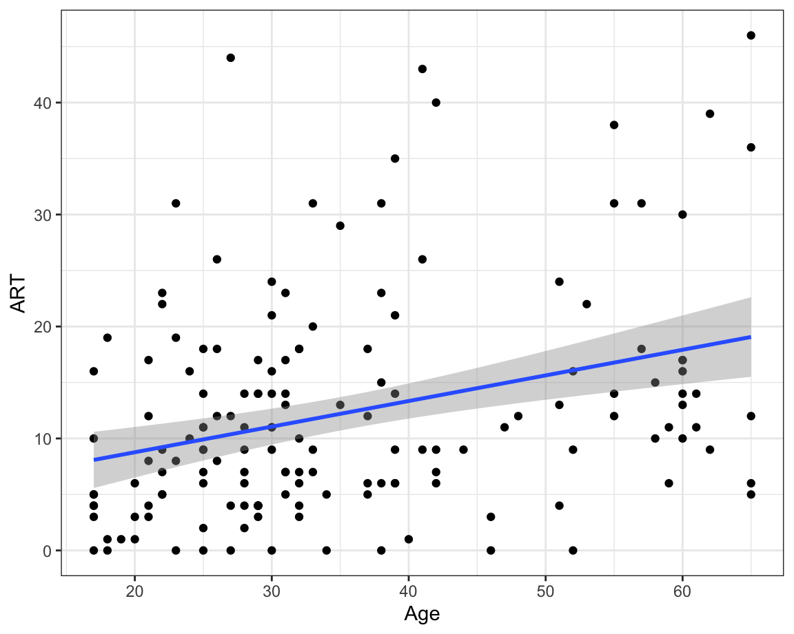
Have you noticed how, having added ART as a predictor to your model, Age no longer makes a statistically significant contribution to the model (p = 0.070994)? How come? Well, it turns out that ART and Age are correlated (r = 0.32, see scatter plot below). This moderate positive correlation makes intuitive sense: the older you are, the more likely you are to have come across more authors and therefore be able to correctly identify them in the Author Recognition Test. Of the two predictors, our model suggests that ART scores are a more useful predictor of Vocab scores than age. In other words, if we know the ART score of a participant from the Dąbrowska (2019) dataset, their age does not provide additional information that can help us to better predict their Vocab score.

Observed relationship between participants’ age and their Author Recognition Test (ART) scores. The blue line shows that there is a moderate positive correlation between these two variables.

Q13.3 What is the predicted Vocab score of a female L1 speaker aged 31 (the median age) with a manual occupation, who scored 16 on the Blocks test (the median score), spent 14 years in formal education (median time period), and scored 20 on the Author Recognition Test?

71.1133
123.3076
8.5405
74.3556
73.6248
74.1007

🐭 Click on the mouse for a hint.

# We must add together the coefficient for the intercept, the coefficient for the manual occupation (which is negative), and the ART coefficient multiplied by 20 (as we did not center this predictor):
62.5728 + -2.5115 + 0.5526*20

Q13.4 By default, the visreg() function displays a 95% confidence band around predicted values, corresponding to a significance level of 0.05. How can you change this default to display a 99% confidence band instead? Run the command ?visreg() to find out how to achieve this from the function’s help file.

visreg(model.ART, xvar = "ART", CI = 0.01)
visreg(model.ART, xvar = "ART", alpha = 0.01)
visreg(model.ART, xvar = "ART", trans = CI(0.99))
visreg(model.ART, xvar = "ART", alpha = "99%")
visreg(model.ART, xvar = "ART", alpha = 99)

🐭 Click on the mouse for a hint.

# The argument that you need to change is called "alpha". This is because the significance level is also called the alpha level (see Section 11.3). 

# The alpha value that corresponds to a 99% confidence interval is equal to:
1 - 0.99

# Hence the code should (minimally) include these arguments:
visreg(model.ART, 
       xvar = "ART", 
       alpha = .01)

Observe how the width of the confidence bands changes when you increase the significance level from 0.01 to 0.1: the higher the significance level, the narrower the confidence band becomes. Remember that the significance level corresponds to the risk that we are willing to take of wrongly rejecting the null hypothesis when it is actually true. Therefore, when we lower this risk by choosing a lower significance level (i.e. 0.01), we end up with wider confidence bands that are more likely to allow us to draw a flat line (see Correlation tests). If we can draw a flat line through a 99% confidence band, this means that we do not have enough evidence to reject the null hypothesis at the significance level of 0.01.

TipYour turn!

In the last Your turn! section, you fitted a multiple linear regression model to predict Vocab scores among L1 and L2 speakers using all of the predictors that we used in model4_c plus ART scores.

Q13.5 Calculate the relative importance of each of the predictors in this model using the {relaimpo} package. What is the relative importance of the predictor ART in this model as estimated by the lmg metric and rounded to two decimal places?

# Fit the model:
model.ART <- lm(Vocab ~ Group + Age_c + OccupGroup + Gender + Blocks_c + EduTotal_c + ART, 
             data = Dabrowska.data)

# Compute the lmg values and extract them as a data frame
library(relaimpo)
rel.imp.metric <- calc.relimp(model.ART, 
                              type = "lmg")

rel.imp.metric.df <- data.frame(lmg = rel.imp.metric$lmg) |> 
    rownames_to_column(var = "Predictor")

rel.imp.metric.df |> 
  mutate(lmg = round(lmg, digits = 2)) |> 
  arrange(-lmg)

TipYour turn!

In this task, we will explore the possibility of an interaction between participants’ native-speaker status (Group) and the number of years they spent in formal education (EduTotal). The underlying idea is that, for the L1 speakers, their formal education will most likely have been in English; hence the longer they were in formal education, the higher they might score on the Vocab test. For the L2 speakers, however, their formal education will more likely have been in a language other than English. As a result, years in formal education may be a weaker predictor of Vocab scores than for L1 speakers.

Q13.6 To begin, generate a plot to visualise this interaction in the observed data: map the EduTotal variable onto the x-axis and Vocab onto the y-axis, and split the plot into two facets, one for L1 and the other for L2 participants. Based on your interpretation of your plot, which of these statements is/are correct?

The number of years that L1 participants spent in formal education is positively correlated with their Vocab scores. This is not the case for L2 participants.
For both L1 and L2 participants, the correlation between the number of years that they spent in formal education and their Vocab scores is not statistically significant.
For both L1 and L2 participants, the number of years that they spent in formal education is positively correlated with their Vocab scores.
For both L1 and L2 participants, the number of years that they spent in formal education is negatively correlated with their Vocab scores.

🐭 Click on the mouse for a hint.

Dabrowska.data |> 
   ggplot(mapping = aes(x = EduTotal, 
                        y = Vocab)) +
     geom_point() +
     facet_wrap(~ Group) +
     geom_smooth(method = "lm", 
                 se = TRUE) +
     theme_bw()

Q13.7 Below is the model formula for model5:

Vocab ~ Group + Age_c + OccupGroup + Gender + Blocks_c + EduTotal_c + Age_c:Group

What do you need to add to this formula to also model the interaction that you just visualised?

+ EduTotal_c:Group
+ EduTotal_c:Group:Vocab
+ Vocab ~ EduTotal_c:Group

Q13.8 Fit the model with the added interaction. Does the interaction make a statistically significant contribution to the model at the significance level of 0.05?

No, it does not.
Yes, it does.

model5.int <- lm(Vocab ~ Group + Age_c + OccupGroup + Gender + Blocks_c + EduTotal_c + Age_c:Group + EduTotal_c:Group,
                 data = Dabrowska.data)

summary(model5.int)

Q13.9 Use the {visreg} package to visualise the interaction effect EduTotal_c:Group as predicted by your model. Looking at your plot of predicted values and partial residuals, which conclusion can you draw?

Years in formal education is a statistically significant predictor of Vocab scores for both L1 and L2 speakers, and there is no striking difference in the strength of this association between the L1 and the L2 group.
Years in formal education is a statistically significant predictor of Vocab scores for L1 speakers, but not L2 speakers.
Years in formal education is a statistically significant predictor of Vocab scores for L2 speakers, but not L1 speakers.
The model makes almost perfect predictions for L1 speakers, but not L2 speakers.
None of these conclusions can be drawn from the plot alone.

🐭 Click on the mouse for a hint.

visreg(model5.int, 
       xvar = "EduTotal_c", 
       by = "Group",
       xtrans = function(x) x + median(Dabrowska.data$EduTotal), 
       gg = TRUE) + 
  labs(x = "Years in formal education",
       y = "Predicted Vocab scores") +
  theme_bw()

TipYour turn!

So far in this chapter, we have fitted a model of L1 speakers’ Vocab scores. We have found that participants’ print exposure (as measured by the ART), non-verbal intelligence (as measured by the Blocks test), their age, the number of years they were in formal education, and the interaction between ART scores and years in education all contribute to being able to predict how well they performed on the Vocab test. The model that we selected as the optimal model (L1.model.back2) was able to predict 58% of the variance in Vocab scores among L1 speakers.

In this task, your aim is to find out which predictors and interactions among predictors can be used to predict Vocab scores among L2 speakers and to what degree of accuracy. In addition to the predictors that we entered in our full L1 model, you can enter three additional predictors in your model that are relevant to L2 speakers only:

• Age at which they started living in an English-speaking country (Arrival)
• Total number of years they have been living in an English-speaking country (LoR)
• Number of hours they spend reading in English in a typical week (ReadEng)

Run the following code to median-center some of these numeric variables in L2.data:

L2.data <- L2.data |> 
  mutate(Blocks_c = Blocks - median(Blocks),
         Age_c = Age - median(Age),
         EduTotal_c = EduTotal - median(EduTotal),
         Arrival_c = Arrival - median(Arrival),
         LoR_c = LoR - median(LoR))

Then, fit the following multiple linear regression model on the L2 dataset and examine the model summary:

L2.model <- lm(formula = Vocab ~ ART + Blocks_c + Age_c + EduTotal_c + Arrival_c + LoR_c + ReadEng + ART:EduTotal_c + ART:ReadEng + EduTotal_c:ReadEng + Arrival_c:Age_c + LoR_c:Arrival_c,
             data = L2.data)

summary(L2.model)

Q13.10 How many interaction terms contribute to the predictions made by L2.model?

0 1 2 3 4 5

🐭 Click on the mouse for a hint.

Q13.11 Use the check_model() function to visually check whether L2.model meets the most important assumptions of multiple linear regression models. Which assumption(s) are obviously violated?

Independence of the data points
Linear relationships between the predictors
Homogeneity of the model residuals
Normality of the model residuals
No overly influential outliers
No multicollinearity
None of these assumptions

🐭 Click on the mouse for a hint.

diagnostic.plots.L2 <- plot(check_model(L2.model, panel = FALSE))

diagnostic.plots.L2[[1]] # No issues here.

diagnostic.plots.L2[[2]] # Also no issues here.

diagnostic.plots.L2[[3]] # Nothing major to worry about: the reference line is not perfectly flat, but it's not far off.

diagnostic.plots.L2[[4]] # No observation points appear to have an overly large influence on the model

diagnostic.plots.L2[[5]] # Here we have three coefficients with VIF scores > 10. This is problematic!

diagnostic.plots.L2[[6]] # The residuals are not normally distributed, but the largest deviation is at lowest end of the distribution which is not terribly unusual.

We can display the exact VIF values of a model using the vif() function from the {car} package (Fox & Weisberg 2018):

install.packages("car")
library(car)

vif(L2.model)

               ART           Blocks_c              Age_c         EduTotal_c 
          5.987790           1.216035          25.347847           5.490682 
         Arrival_c              LoR_c            ReadEng     ART:EduTotal_c 
         23.746278          11.102277           3.661388           2.237536 
       ART:ReadEng EduTotal_c:ReadEng    Age_c:Arrival_c    Arrival_c:LoR_c 
          8.550867           4.412402           3.349661           1.398937 

From this list of VIF values, we can see that three predictors display high collinearity: Age_c, Arrival_c, and LoR_c. This makes sense because, for most L2 participants recruited in the UK, if we know how old they were when they arrived in the UK (Arrival), and their length of residence in the country in years (LoR), then we can probably almost predict their age (Age) to a high degree of accuracy. We can easily check this hypothesis in a random sample of six participants from our L2.data:

L2.data |> 
  select(Arrival, LoR, Age) |> 
  slice_sample(n = 6)

  Arrival LoR Age
1      26   3  29
2      32   6  38
3      22   5  28
4      17   3  20
5      23   4  27
6      16  14  30

As you can see, in most cases, participants’ age is equal to their age when they first arrived in the country plus the number of years they’ve been living there since. This is why Age and the combination of the predictors Arrival and LoR are almost perfectly correlated:

cor(L2.data$Age, (L2.data$Arrival + L2.data$LoR))

[1] 0.9768833

To remedy this, we must remove one of these three predictors from our model. Fit a new model that does not include participants’ age when they first arrived in the UK (Arrival). Save this new model as L2.model.b. Check that it now meets all the model assumptions and then examine its summary.

Q13.12 Adjusted for the number of predictors entered into L2.model.b, what percentage of the variance in Vocab scores in the L2 dataset does this model accurately predict?

Practically 0% About 3% About 15% About 20% About 22% About 31% About 57%

L2.model.b <- lm(formula = Vocab ~ ART + Blocks_c + Age_c + EduTotal_c + LoR_c + ReadEng + ART:EduTotal_c + ART:ReadEng + EduTotal_c:ReadEng,
             data = L2.data)

check_model(L2.model.b) # Now all looking much better than earlier!

summary(L2.model.b) # Adjusted R-squared:  0.2027

Q13.13 Which main-effect predictor(s) make a statistically significant contribution to L2.model.b at α = 0.05?

ART
Blocks_c
Age_c
EduTotal_c
Arrival_c
LoR_c
ReadEng

Q13.14 Does the model’s coefficient estimate for ReadEng make intuitive sense?

Yes, the ReadEng coefficient is positive, which means that the more time L2 speakers regularly spend reading in English, the higher their predicted receptive English vocabulary test scores.
No, the ReadEng coefficient is larger than all other coefficients, which violates the model assumption of no overly influential outliers.

Q13.15 Which interaction effect(s) make a statistically significant contribution to L2.model.b at α = 0.05?

ART:EduTotal_c
ART:ReadEng
EduTotal_c:ReadEng
None of them

Q13.16 Use the {visreg} library to visualise the model’s predicted Vocab scores (on the y-axis) as a function of all possible ReadEng values (on the x-axis) and subdivide the figure into three panels corresponding to low, mid-level, and high ART scores. Which arguments do you have to use inside the visreg() function to achieve this?

fit = L2.model.b
xvar = "ART"
xvar = "ReadEng"
xtrans = function(x) x + median(L2.data$ReadEng)
by = "ReadEng"
by = "ART"

🐭 Click on the mouse for a hint.

visreg(fit = L2.model.b,
       xvar = "ReadEng",
       by = "ART")

Check your progress 🌟

Congratulations: you have successfully completed the most difficult chapter of this textbook! 💪 You have answered 0 out of 16 questions correctly.

Acheson, Daniel J., Justine B. Wells & Maryellen C. MacDonald. 2008. New and updated tests of print exposure and reading abilities in college students. Behavior Research Methods 40(1). 278–289. https://doi.org/10.3758/brm.40.1.278.

Dąbrowska, Ewa. 2019. Experience, aptitude, and individual differences in linguistic attainment: A comparison of native and nonnative speakers. Language Learning 69(S1). 72–100. https://doi.org/10.1111/lang.12323.

Fox, John & Sanford Weisberg. 2018. An R companion to applied regression. 3. edn. Los Angeles London New Delhi Singapore Washington, DC Melbourne: SAGE.